GCP – Zero-shot forecasting in BigQuery with the TimesFM foundation model
Accurate time-series forecasting is essential for many business scenarios such as planning, supply chain management, and resource allocation. BigQuery now embeds TimesFM, a state-of-the-art pre-trained model from Google Research, enabling powerful forecasting via the simple AI.FORECAST function.
Time-series analysis is used across a wide range of fields including retail, healthcare, finance, manufacturing, and the sciences. Through the use of forecasting algorithms, users can have a more thorough understanding of their data including the recognition of trends, seasonal variations, cyclical patterns, and stationarity.
BigQuery already natively supports the well-known ARIMA_PLUS and ARIMA_PLUS_XREG models for time-series analysis. More recently, with the rapid progress and success of large pre-trained LLM models, the Google Research team developed TimesFM, a foundational model specifically for the time series domain.
The Time Series foundation model
TimesFM is a forecasting model that’s pre-trained on a large time-series corpus of 400 billion real-world time-points. A big advantage of this model is its ability to perform “zero-shot” forecasting. This means that it can make accurate predictions on unseen datasets without any training. In terms of the architecture, TimesFM is built as a decoder-only transformer model, which outputs batches of contiguous time-point segments at a time. This model has been featured on the GIFT-Eval benchmark and Monash public dataset, with a variety of public benchmarks from different domains and granularities. While ARIMA_PLUS offers customizability and explainability, the TimesFM model provides high ease-of-use and delivers good generalizability across many business domains, and often beats custom trained statistical and deep learning models.
- aside_block
- <ListValue: [StructValue([(‘title’, ‘$300 in free credit to try Google Cloud data analytics’), (‘body’, <wagtail.rich_text.RichText object at 0x3e0672d0b550>), (‘btn_text’, ‘Start building for free’), (‘href’, ‘http://console.cloud.google.com/freetrial?redirectPath=/bigquery/’), (‘image’, None)])]>
How BigQuery supports TimesFM
The latest TimesFM 2.0 is now a native model in BigQuery. With 500 million parameters, TimesFM model inference runs directly on BigQuery infrastructure so there are no models to train, endpoints to manage, connections to set up, or quotas to adjust. TimesFM in BigQuery is also fast and scalable — you can forecast millions of univariate time series in a few minutes with a single SQL query.
Examples of the new AI.FORECAST function
To demonstrate, consider a use case that relies on the public bigquery-public-data.san_francisco_bikeshare.bikeshare_trips table. This dataset contains information about individual bicycle trips taken using the San Francisco Bay Area’s bike-share program.
Example 1: Single time series
The following query aggregates the total number of bike-share trips on each day and forecasts the number of trips for the next 10 days (the default horizon).
- code_block
- <ListValue: [StructValue([(‘code’, “SELECT *rnFROMrn AI.FORECAST(rn (rn SELECT TIMESTAMP_TRUNC(start_date, DAY) AS trip_date, COUNT(*) AS num_tripsrn FROM `bigquery-public-data.san_francisco_bikeshare.bikeshare_trips`rn GROUP BY 1rn ),rn timestamp_col => ‘trip_date’,rn data_col => ‘num_trips’);”), (‘language’, ‘lang-sql’), (‘caption’, <wagtail.rich_text.RichText object at 0x3e0672d0b700>)])]>
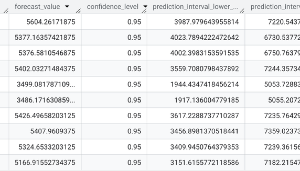
The results look similar to:

The output includes the forecast timestamp and values through the columns forecast_timestamp and forecast_value. The confidence_level is default as 0.95. The prediction_interval_lower_bound and prediction_interval_upper_bound show the bounds for each forecasted point.
Example 2: Multiple time series
The AI.FORECAST function also lets you forecast multiple time series at a time as shown in the following example. The following query forecasts the number of bike share trips per subscriber type and per hour for the next month (approximately 720 hours), based on the previous four months of historical data.
- code_block
- <ListValue: [StructValue([(‘code’, “SELECT *rnFROMrn AI.FORECAST(rn (rn SELECTrn TIMESTAMP_TRUNC(start_date, HOUR) AS trip_hour,rn subscriber_type,rn COUNT(*) AS num_tripsrn FROM `bigquery-public-data.san_francisco_bikeshare.bikeshare_trips`rn WHERE start_date >= TIMESTAMP(‘2018-01-01’)rn GROUP BY 1, 2rn ),rn horizon => 720,rn timestamp_col => ‘trip_hour’,rn data_col => ‘num_trips’,rn id_cols => [‘subscriber_type’]);”), (‘language’, ‘lang-sql’), (‘caption’, <wagtail.rich_text.RichText object at 0x3e06468ee4f0>)])]>
The results look similar to the following:

In addition to the columns used by the single time series, there’s the time series identifier column, which we defined earlier as subscriber_type.Visualize the results
You can merge the history data and forecasted data and visualize these results. The following graph visualizes the ‘Subscriber’ time series with its the lower and upper bounds of the prediction interval as follows:

You can see the detailed queries we used to generate this in the tutorial.
When to use TimesFM vs ARIMA_PLUS
For quick, out-of-the-box forecasts, establishing baselines, or identifying general trends with minimal setup, use TimesFM. If you need to model specific patterns, fine-tune forecasts for seasonality or holidays, multivariate (ARIMA_PLUS_XREG), require explainable results, or want to leverage a longer historical context, ARIMA_PLUS is the more suitable choice.
Take the next step
The TimesFM 2.0 model is now available in BigQuery in preview. For more details, please see the tutorial and the documentation.
Read More for the details.


