GCP – Why Stochastic Rounding is Essential for Modern Generative AI

In computing’s early days of the 1940s, mathematicians discovered a flawed assumption about the behavior of round-off errors. Instead of canceling out, fixed-point arithmetic accumulated errors, compromising the accuracy of calculations. A few years later, “random round-off” was proposed, which would round up or down based on a random probability proportional to the remainder.

In today’s age of generative AI, we face a new numerical challenge. To overcome memory bottlenecks, the industry is shifting to lower precision formats like FP8 and emerging 4-bit standards. However, training in low precision is fragile. Standard rounding destroys the tiny gradient updates driving learning, causing model training to stagnate. That same technique from the 1950s, now known as stochastic rounding, is allowing us to train massive models without losing the signal. In this article, you’ll learn how frameworks like JAX and Qwix apply this technique on modern Google Cloud hardware to make low-precision training possible.

When Gradients Vanish

The challenge in low-precision training is vanishing updates. This occurs when small gradient updates are systematically rounded to zero by “round to nearest” or RTN arithmetic. For example, if a large weight is 100.0 and the learning update is 0.001, a low-precision format may register 100.001 as identical to 100.0. The update effectively vanishes, causing learning to stall.

Let’s consider the analogy of a digital swimming pool that only records the water level in whole gallons. If you add a teaspoon of water, the system rounds the new total back down to the nearest gallon. This effectively deletes your addition. Even if you pour in a billion teaspoons one by one, the recorded water level never rises.

Precision through Probability

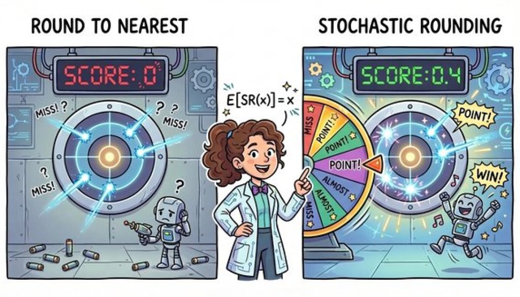
Stochastic rounding, or SR for short, solves this by replacing deterministic rounding rules with probability. For example, instead of always rounding 1.4 down to 1, SR rounds it to 1 with 60% probability and 2 with 40% probability.

Mathematically, for a value x in the interval [⌊x⌋,⌊x⌋+1], the definition is:

The defining property is that SR is unbiased in expectation:

• Stochastic Rounding: E[SR(x)] = x

• Round-to-Nearest: E[RTN(x)] ≠ x

To see the difference, look at our 1.4 example again. RTN is deterministic: it outputs 1 every single time. The variance is 0. It is stable, but consistently wrong. SR, however, produces a noisy stream like 1, 1, 2, 1, 2.... The average is correct (1.4), but the individual values fluctuate.

We can quantify the “cost” of zero bias with the variance formula:

Var(SR(x))=p(1-p) where p=x-⌊x⌋

In contrast, RTN has zero variance, but suffers from fast error accumulation. In a sum of N operations, RTN’s systematic error can grow linearly (O(N)). If you consistently round down by a tiny amount, those errors stack up fast.

SR behaves differently. Because the errors are random and unbiased, they tend to cancel each other out. This “random walk” means the total error grows only as the square root of the number of operations O(√N).

While stochastic rounding introduces noise, the tradeoff can often be benign. In deep learning, this added variance often acts as a form of implicit regularization, similar to dropout or normalization, helping the model escape shallow local minima and generalize better.

Implementing on Google Cloud

Google Cloud supports stochastic rounding through its latest generation of AI accelerators, including Cloud TPUs and NVIDIA Blackwell GPUs. These accelerators can also be used in AI-optimized Google Kubernetes Engine clusters.

Native Support on TPUs

Google’s TPU architecture includes native hardware support for stochastic rounding in the Matrix Multiply Unit (MXU). This allows you to train in lower-precision formats like INT4, INT8 and FP8 without meaningful degradation of model performance.

You can use Google’s Qwix library, a quantization toolkit for JAX that supports both training (QAT) and post-training quantization (PTQ). Here is how you might configure it to quantize a model in INT8, explicitly enabling stochastic rounding for the backward pass to prevent vanishing updates:

Qwix abstracts the complexity of low-level hardware instructions, allowing you to inject quantization logic directly into your model’s graph with a simple configuration.

NVIDIA Blackwell & A4X VMs

The story is similar if you are using NVIDIA GPUs on Google Cloud. You can deploy A4X VMs, the industry’s first cloud instance powered by the NVIDIA GB200 NVL72 system. These VMs connect 72 Blackwell GPUs into a single supercomputing unit, the AI Hypercomputer.

Blackwell introduces native hardware support for NVFP4, a 4-bit floating-point format that utilizes a block scaling strategy. To preserve accuracy, the NVFP4BlockScaling recipe automatically applies stochastic rounding to gradients to avoid bias, along with other advanced scaling techniques.

When you wrap your layers in te.autocast with this recipe, the library engages these modes for the backward pass:

By simply entering this context manager, the A4X’s GB200 GPUs perform matrix multiplications in 4-bit precision while using stochastic rounding for the backward pass, delivering up to 4x higher training performance than previous generations without compromising convergence.

Best Practices for Production

To effectively implement SR in production, first remember that stochastic rounding is designed for training only. Because it is non-deterministic, you should stick to standard Round-to-Nearest for inference workloads where consistent outputs are required.

Second, use SR as a tool for debugging divergence. If your low-precision training is unstable, check your gradient norms. If they are vanishing, enabling SR may help, while exploding gradients suggest problems elsewhere.

Finally, manage reproducibility carefully. Since SR relies on random number generation, bit-wise reproducibility is more challenging. Always set a global random seed, for example, using jax.random.key(0), to ensure that your training runs exhibit “deterministic randomness,” producing the same results each time despite the internal probabilistic operations.

Stochastic rounding transforms the noise of low-precision arithmetic into the signal of learning. Whether you are pushing the boundaries with A4X VMs or Ironwood TPUs, this 1950’s numerical method is the key to unlocking the next generation of AI performance.

Connect on LinkedIn, X, and Bluesky to continue the discussion about the past, present, and future of AI infrastructure.