GCP – Event-triggered detection of data drift in ML workflows
With ML workflows, it is often insufficient to train and deploy a given model just once. Even if the model has desired accuracy initially, this can change if the data used for making prediction requests becomes—perhaps over time—sufficiently different from the data used to originally train the model.
When new data becomes available, which could be used for retraining a model, it can be helpful to apply techniques for analyzing data ‘drift’, and determining whether the drift is sufficiently anomalous to warrant retraining.
It can also be useful to trigger such an analysis—and potential re-run of your training pipeline—automatically, upon arrival of new data.
This blog post highlights an example notebook that shows how to set up such a scenario with Kubeflow Pipelines (KFP).
It shows how to build a pipeline that checks for statistical drift across successive versions of a dataset and uses that information to make a decision on whether to (re)train a model; and how to configure event-driven deployment of pipeline jobs when new data arrives. (In this example, we show full model retraining on a new dataset. An alternate scenario—not covered here—could involve tuning an existing model with new data.)
The notebook builds on an example highlighted in a previous blog post—which shows a KFP training and serving pipeline—and introduces two primary new concepts:
- The example demonstrates use of the TensorFlow Data Validation (TFDV) library to build pipeline components that derive dataset statistics and detect drift between older and newer dataset versions, and shows how to use drift information to decide whether to retrain a model on newer data.
- The example shows how to support event-triggered launch of Kubeflow Pipelines runs from a Cloud Functions (GCF) function, where the Function run is triggered by addition of a file to a given Cloud Storage (GCS) bucket.
The machine learning task uses a tabular dataset that joins London bike rental information with weather data, and trains a Keras model to predict rental duration. See this and this blog post and associated README for more background on the dataset and model architecture.
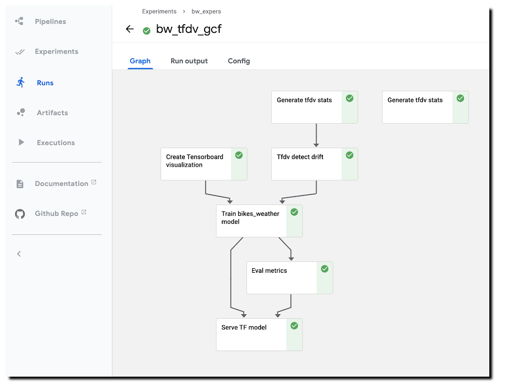
A pipeline run using TFDV-based components to detect ‘data drift’.
Running the example notebook
The example notebook requires a Google Cloud Platform (GCP) account and project, ideally with quota for using GPUs, and—as detailed in the notebook—an installation of AI Platform Pipelines (Hosted Kubeflow Pipelines) (that is, an installation of KFP on Google Kubernetes Engine (GKE)), with a few additional configurations once installation is complete.
The notebook can be run using either Colab (open directly) or AI Platform Notebooks (open directly).
Creating TFDV-based KFP components
Our first step is to build the TFDV components that we want to use in our pipeline.
Note: For this example, our training data is in GCS, in CSV-formatted files. So, we can take advantage of TFDV’s ability to process CSV files. The TFDV libraries can also process files in TFRecords format.
We’ll define both TFDV KFP pipeline components as ‘lightweight’ Python-function-based components. For each component, we define a function, then call kfp.components.func_to_container_op() on that function to build a reusable component in .yaml format.
Let’s take a closer look at how this works (details are in the notebook).
Below is the Python function we’ll use to generate TFDV statistics from a collection of csv files. The function—and the component we’ll create from it—outputs the path to the generated stats file. When we define a pipeline that uses this component, we’ll use this step’s output as input to another pipeline step.
TFDV uses a Beam pipeline—not to be confused with KFP Pipelines—to implement the stats generation. Depending upon configuration, the component can use either the Direct (local) runner or the Dataflow runner. Running the Beam pipeline on Dataflow rather than locally can make sense with large datasets.
To turn this function into a KFP component, we’ll call kfp.components.func_to_container_op(). We’re passing it a base container image to use: gcr.io/google-samples/tfdv-tests:v1. This base image has the TFDV libraries already installed, so that we don’t need to install them ‘inline’ when we run a pipeline step based on this component.
We’ll take the same approach to build a second TFDV-based component, one which detects drift between datasets by comparing their stats. The TFDV library makes this straightforward. We’re using a drift comparator appropriate for a regression model—as used in the example pipeline—and looking for drift on a given set of fields (in this case, for example purposes, just one).
The tensorflow_data_validation.validate_statistics() call will then tell us whether the drift anomaly for that field is over the specified threshold. See the TFDV docs for more detail.
(The details of this second component definition are in the example notebook).
Defining a pipeline that uses the TFDV components
After we’ve defined both TFDV components—one to generate stats for a dataset, and one to detect drift between datasets—we’re ready to build a Kubeflow Pipeline that uses these components, in conjunction with previously-built components for a training & serving workflow.
Instantiate pipeline ops from the components
KFP components in yaml format are shareable and reusable. We’ll build our pipeline by starting with some already-built components—(described in more detail here)—that support our basic ‘train/evaluate/deploy’ workflow.
We’ll instantiate some pipeline ops from these pre-existing components like this, by loading them via URL:
Then, we define a KFP pipeline from the defined ops. We’re not showing the pipeline in full here—see the notebook for details.
Two pipeline steps are based on the tfdv_op, which generates the stats. tfdv1 generates stats for the test data, and tfdv2 for the training data.
In the following, you can see that the tfdv_drift step (based on the tfdv_drift_op) takes as input the output from the tfdv2 (stats for training data) step.
While not all pipeline details are shown, you can see that this pipeline definition includes some conditional expressions; parts of the pipeline will run only if an output of an ‘upstream’ step meets the given conditions. We start the model training step if drift anomalies are detected. (And, once training is completed, we’ll deploy the model for serving only if its evaluation metrics meet certain thresholds.)
Here’s the DAG for this pipeline. You can see the conditional expressions reflected; and can see that the step to generate stats for the test dataset provides no downstream dependencies, but the stats on the training set are used as input for the drift detection step.
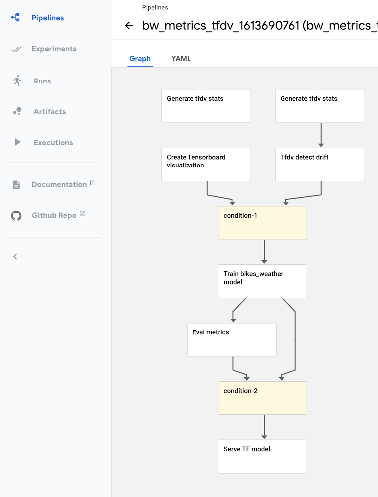
The pipeline DAG
Here’s a pipeline run in progress:
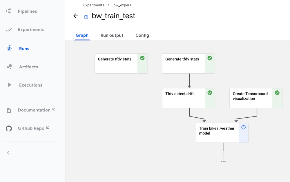
A pipeline run in progress.
See the example notebook for more details on how to run this pipeline.
Event-triggered pipeline runs
Once you have defined this pipeline, a next useful step is to automatically run it when an update to the dataset is available, so that each dataset update triggers an analysis of data drift and potential model (re)training.
We’ll show how to do this using Cloud Functions (GCF), by setting up a function that is triggered when new data is added to a GCS bucket.
Set up a GCF function to trigger a pipeline run when a dataset is updated
We’ll define and deploy a Cloud Functions (GCF) function that launches a run of this pipeline when new training data becomes available, as triggered by the creation or modification of a file in a ‘trigger’ bucket on GCS.
In most cases, you don’t want to launch a new pipeline run for every new file added to a dataset—since typically, the dataset will consist of a collection of files, to which you will add/update multiple files in a batch. So, you don’t want the ‘trigger bucket’ to be the dataset bucket (if the data lives on GCS)—as that will trigger unwanted pipeline runs.
Instead, we’ll trigger a pipeline run after the upload of a batch of new data has completed.
To do this, we’ll use an approach where the ‘trigger’ bucket is different from the bucket used to store dataset files. ‘Trigger files’ uploaded to that bucket are expected to contain the path of the updated dataset as well as the path to the data stats file generated for the last model trained.
A trigger file is uploaded once the new data upload has completed, and that upload triggers a run of the GCF function, which in turn reads info on the new data path from the trigger file and launches the pipeline job.
Define the GCF function
To set up this process, we’ll first define the GCF function in a file called main.py, as well as an accompanying requirements file in the same directory that specifies the libraries to load prior to running the function. The requirements file will indicate to install the KFP SDK:
kfp==1.4
The code looks like this (with some detail removed); we parse the trigger file contents and use that information to launch a pipeline run. The code uses the values of several environment variables that we will set when uploading the GCF function.
Then we’ll deploy the GCF function as follows. Note that we’re indicating to use the gcs_update definition (from main.py), and specifying the trigger bucket. Note also how we’re setting environment vars as part of the deployment.
Trigger a pipeline run when new data becomes available
Once the GCF function is set up, it will run when a file is added to (or modified in) the trigger bucket. For this simple example, the GCF function expects trigger files of the following format, where the first line is the path to the updated dataset, and the second line is the path to the TFDV stats for the dataset used for the previously-trained model. More generally, such a trigger file can contain whatever information is necessary to determine how to parameterize the pipeline run.
gs://path/to/new/or/updated/dataset/
gs://path/to/stats/from/previous/dataset/stats.pb
What’s next?
This blog post showed how to build Kubeflow Pipeline components, using the TFDV libraries, to analyze datasets and detect data drift. Then, it showed how to support event-triggered pipeline runs via Cloud Functions.
The post didn’t include use of TFDV to visualize and explore the generated stats, butthis example notebook shows how you can do that.
You can alsoexplore the samples in the Kubeflow Pipelines GitHub repo.
Read More for the details.
