GCP – Benchmarking rendering software on Compute Engine
For our customers who regularly perform rendering workloads such as animation or visual effects studios, there is a fixed amount of time to deliver a project. When faced with a looming deadline, these customers can leverage cloud resources to temporarily expand their fleet of render servers to help complete work within a given timeframe, a process known as burst rendering. To learn more about deploying rendering jobs to Google Cloud, see Building a Hybrid Render Farm.
When gauging render performance on the cloud, customers sometimes reproduce their on-premises render worker configurations by building a virtual machine (VM) with the same number of CPU cores, processor frequency, memory, and GPU. While this may be a good starting point, the performance of a physical render server is rarely equivalent to a VM running on a public cloud with a similar configuration. To learn more about comparing on-premises hardware to cloud resources, see the reference article Resource mappings from on-premises hardware to Google Cloud.
With the flexibility of cloud, you canright-size your resources to match your workload. You can define each individual resource to complete a task within a certain time, or within a certain budget.
But as new CPU and GPU platforms are introduced or prices change, this calculation can become more complex. How can you tell if your workload would benefit from a new product available on Google Cloud?
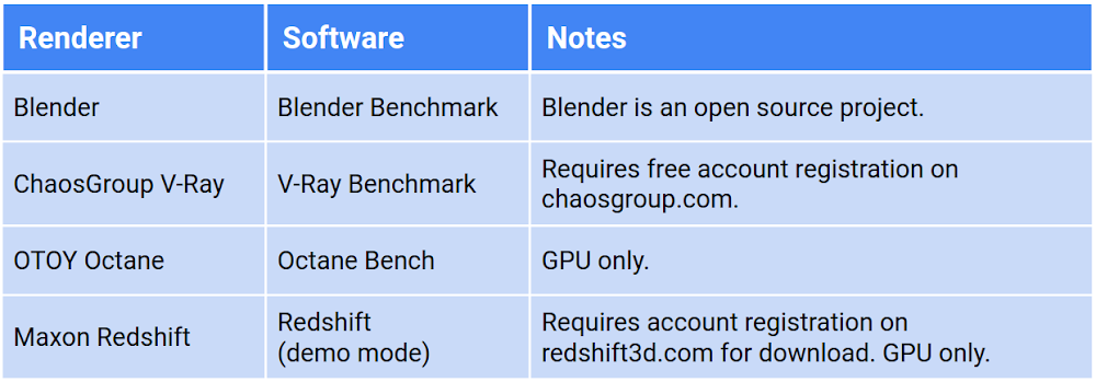
This article examines the performance of different rendering software on Compute Engine instances. We ran benchmarks for popular rendering software across all CPU and GPU platforms, across all machine type configurations to determine the performance metrics of each. The render benchmarking software we used is freely-available from a variety of vendors. You can see a list of the software we used in the table below, and learn more about each in Examining the benchmarks.
Note: Benchmarking of any render software is inherently biased towards the scene data included with the software and the settings chosen by the benchmark author. You may want to run benchmarks with your own scene data within your own cloud environment to fully understand how to take advantage of the flexibility of cloud resources.
Benchmark overview
Render benchmark software is typically provided as a standalone executable containing everything necessary to run the benchmark: a license-free version of the rendering software itself, the scene or scenes to render, and supporting files are all bundled in a single executable that can be run either interactively or from a command line.
Benchmarks can be useful for determining the performance capabilities of your configuration when compared to other posted results. Benchmarking software such as Blender Benchmark use job duration as their main metric; the same task is run for each benchmark no matter the configuration. The faster the task completes, the higher the configuration is rated.
Other benchmarking software such as V-Ray Bench examines how much work can be completed during a fixed amount of time. The amount of computations completed by the end of this time period provides the user with a benchmark score that can be compared to other benchmarks.
Benchmarking software is subject to the limitations or features of the renderer on which they’re based. For example, software such as Octane or Redshift cannot take advantage of CPU-only configurations as they’re both GPU-native renderers. V-Ray from ChaosGroup can take advantage of both CPU and GPU but performs different benchmarks depending on the accelerator, and therefore cannot be compared to each other.
We tested the following render benchmarks:
Choosing instance configurations
An instance on Google Cloud can be made up of almost any combination of CPU, GPU, RAM, and disk. In order to gauge performance across a large number of variables, we defined how to use each component and locked its value when necessary for consistency. For example, we let the machine type determine how much memory was assigned to each VM, and we created each machine with a 10 GB boot disk.
Number and type of CPU
Google Cloud offers a number of CPU platforms from different manufacturers. Each platform (referred to as Machine Type in the Console and documentation) offers a range of options, from a single vCPU all the way up to the m2-megamem-416. Some platforms offer different generations of CPUs, and new generations are introduced on Google Cloud as they come on the market.
We limited our research to predefined machine types on N1, N2, N2D, E2, C2, M1, and M2 CPU platforms. All benchmarks were run on a minimum of 4 vCPUs, using the default amount of memory allocated to each predefined machine type.
Number and type of GPU
For GPU-accelerated renderers, we ran benchmarks across all combinations of all NVIDIA GPUs available on Google Cloud. To simplify GPU renderer benchmarks, we used only a single, predefined machine type, the n1-standard-8, as most GPU renderers don’t take advantage of CPUs for rendering (with the exception of V-Ray’s Hybrid Rendering feature, which we didn’t benchmark for this article).
Not all GPUs have the same capabilities: some GPUs support NVIDIA’s RTX, which can accelerate certain raytracing operations for some GPU renderers. Other GPUs offer NVLink, which supports faster GPU-to-GPU bandwidth and offers a unified memory space across all attached GPUs. The rendering software we tested works across all GPU types, and is able to leverage these types of unique features, if available.
For all GPU instances we installed NVIDIA driver version 460.32.03, available from NVIDIA’s public download driver page as well as from our public cloud bucket. This driver runs CUDA Toolkit 11.2, and supports features of the new Ampere architecture of the A100’s.
Note: Not all GPU types are available in all regions. To view available regions and zones for GPUs on Compute Engine, see GPUs regions and zone availability.
Type and size of boot disk
All render benchmark software we used takes up less than a few GB of disk, so we kept the boot disk for each test instance as small as possible. To minimize cost, we chose a boot disk size of 10 GB for all VMs. A disk of this size will only deliver modest performance, but rendering software typically ingest scene data into memory prior to running the benchmark; disk I/O has little effect on the benchmark.
Region
All benchmarks were run in the us-central1 region. We located instances in different zones within the region, based on resource availability.
Note: Not all resource types are available in all regions. To view available regions and zones for CPUs on Compute Engine, see available regions and zones. To view available regions and zones for GPUs on Compute Engine, see GPUs regions and zone availability.
Calculating benchmark costs
All prices in this article are calculated inclusive of all instance resources (CPU, GPU, memory, and disk) for only the duration of the benchmark itself. Each instance incurs startup time, driver and software installation, and latency prior to shutdown following the benchmark. We didn’t add this extra time to the costs shown, which could be reduced by baking an image or by running within a container.
Prices are current at the time of writing, based on resources in the us-central1 region, and are in USD. All prices are for on-demand resources; most rendering customers will want to use preemptible VMs, which are well-suited for rendering workloads, but for the purposes of this article it’s more important to see the relative differences between resources than overall cost. See the Google Cloud Pricing Calculator for more details.
To come up with hourly costs for each machine type, we added together the various resources that make up each configuration:
cost/hr = vCPUs + RAM (GB) + boot disk (GB) + GPU (if any)
To get the cost of an individual benchmark, we multiplied the duration of the render by this cost/hr:
total cost = cost/hr * render duration
Cost performance index
Calculating cost based on how long a render takes only works for benchmarks that use render duration as a metric. Other benchmarks such as V-Ray and Octane calculate a score by measuring the amount of computations possible within a fixed period of time. For these benchmarks, we calculate the Cost Performance Index (CPI) of each render, which can be expressed as:
CPI = Value / Cost
For our purposes, we substitute Value with Score, and Cost with the hourly cost of the resources:
CPI = score / cost/hr
This gives us a single metric that represents both price and the performance of each instance configuration.
Calculating CPI in this manner makes it easy to compare results to each other within a single renderer; the resulting values themselves aren’t as important as how they compare to other configurations running the same benchmark.
For example, examine the CPI of three different configurations rendering the V-Ray Benchmark:

To make these values easier to comprehend, we can normalize them by defining a pivot point; a target resource configuration that has a CPI of 1.0. In this example, we use n1-standard-8 as our target resource:
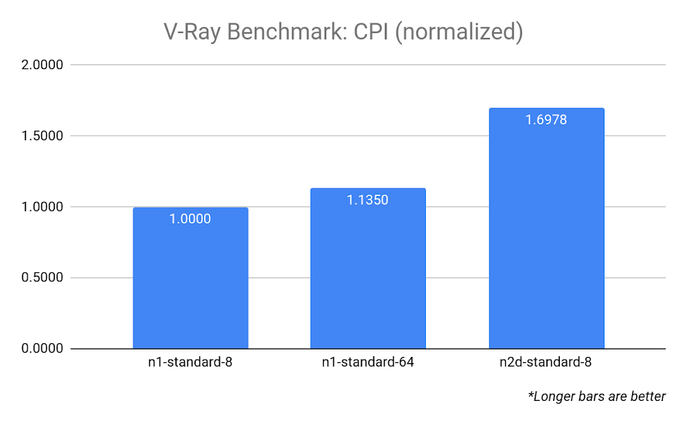
This makes it easier to see that the n2d-standard-8 has a CPI that’s around 70% higher than that of the n1-standard-8.
For CPU benchmarks, we defined the target resource as an n1-standard-8. For GPU benchmarks, we defined the target resource as an n1-standard-8 with a single NVIDIA P100. A CPI greater than 1.0 indicates better cost/performance compared to the target resource, and CPI less than 1.0 indicates lower cost/performance compared to the target resource.
For formula for calculating CPI using the target resource can be expressed as:
CPI = (score / cost/hr) / (target-score / target-cost/hr)
We use CPI in the Examining the benchmarks section.
Comparing instance configurations
Our first benchmark examines the performance differences between a number of predefined N1 machine type configurations. When we run the Blender Benchmark on a selection of six configurations and compare duration and the cost to perform the benchmark (cost/hr x duration), we see an interesting result:
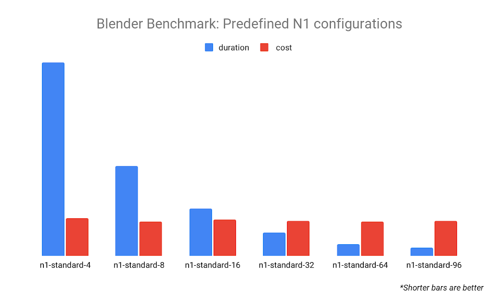
The cost for each of these benchmarks is almost identical, but the duration is dramatically different. This tells us that the Blender renderer scales well as we increase the number of CPU resources. For a Blender render, if you want to get your results back quickly, it makes sense to choose a configuration with more vCPUs.
When we compare the N1 CPU platform to other CPU platforms, we learn even more about Blender’s rendering software. Compare the Blender Benchmark across all CPU platforms with 16 vCPUs:
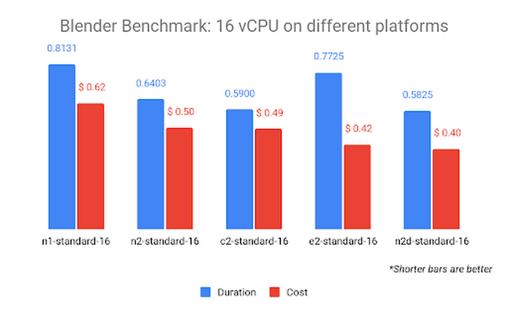
The graph above is sorted according to cost, with least expensive on the right. The N2D CPU platform (which uses AMD EPYC Rome CPUs) is the lowest cost and completes the benchmark in the shortest amount of time. This may indicate that Blender can render more efficiently on AMD CPUs, a fact that can also be observed on their public benchmark results page. The C2 CPU platform (which uses Intel Cascade Lake CPUs) comes in a close second, possibly because it offers the highest sustained frequency of 3.9 GHz.
Note: While a few pennies’ difference may seem trivial for a single render test, a typical animated feature is 90 minutes (5400 seconds) in duration. At 24 frames per second, that’s approximately 130,000 frames to be rendered for a single iteration. Some elements can go through tens or even hundreds of iterations before final approval. A miniscule difference at this scale can mean a massive difference in cost by the end of a production.
CPU vs GPU
Blender Benchmark allows you to compare CPU and GPU performance using the same scenes and metrics. The advantage of GPU rendering is revealed when we compare the previous CPU results to that of a single NVIDIA T4 GPU:
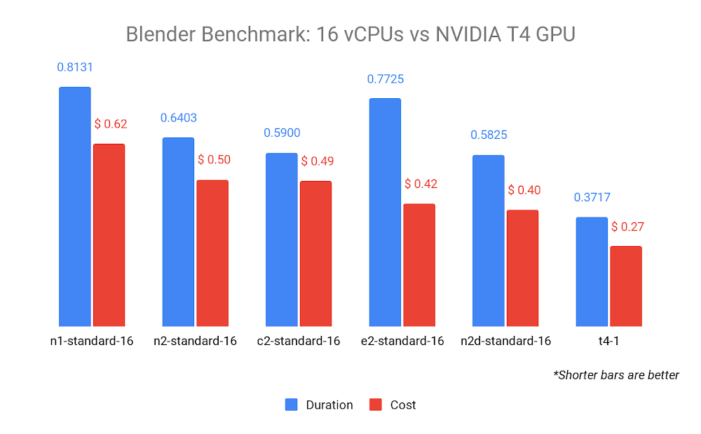
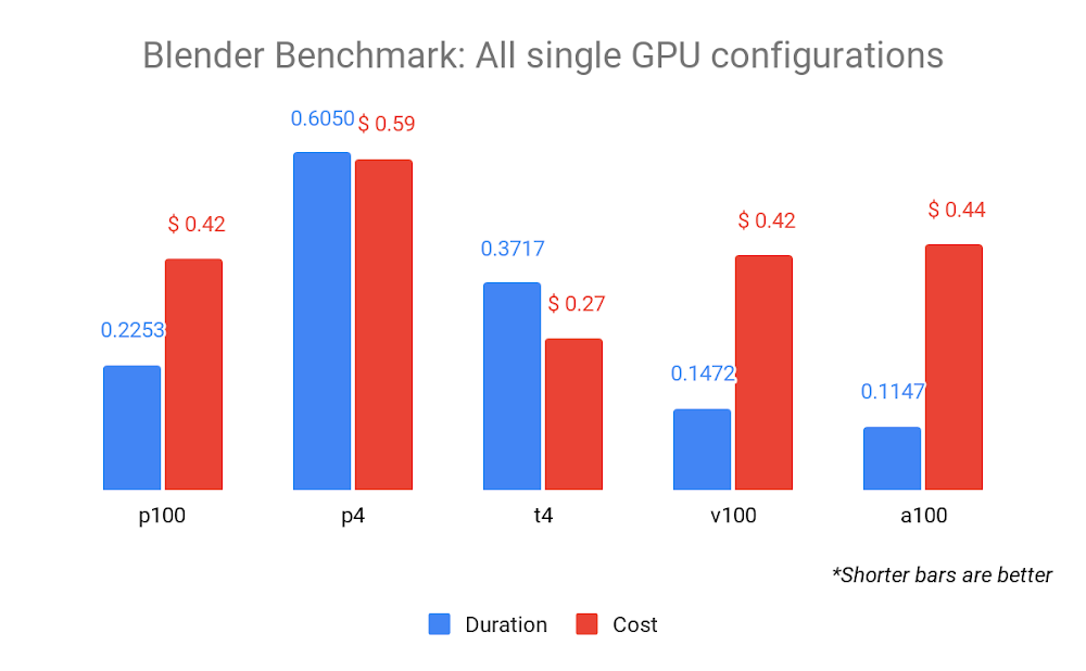
The Blender Benchmark is both faster and cheaper when run in GPU mode on an n1-standard-8 with a single NVIDIA T4 GPU attached. When we run the benchmark on all GPU types, the results can vary widely in both cost and duration:
GPU performance
Some GPU configurations have a higher hourly cost, but their performance specifications give them a better cost-to-performance advantage than lower-cost resources.
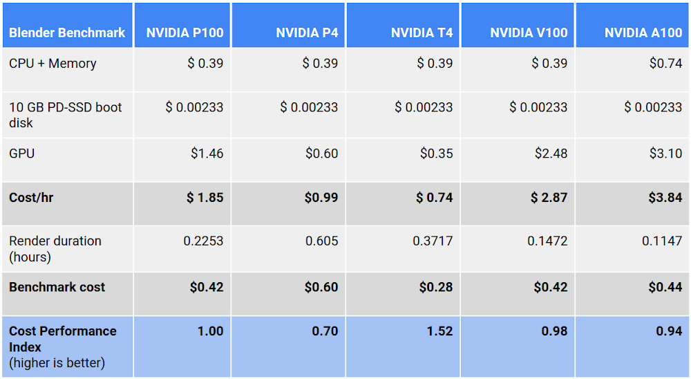
For example, the FP64 performance of the NVIDIA Tesla A100 (9.7 TFLOPS) is 38 times higherthan that of the T4 (0.25 TFLOPS), yet the A100 is around 9 times the cost. In the above diagram, the P100, V100, and A100 cost almost the same, yet the A100 finished the render almost twice as fast as the P100.
By far the most cost-effective GPU in the fleet is the NVIDIA T4, but it didn’t outperform the P100, V100, or A100 for this particular benchmark.
All GPU benchmarks (except the A100, which used the a2-highgpu-1g configuration) used the n1-standard-8 configuration with a 10 GB PD-SSD boot disk:
We can also examine how the same benchmark performs on an instance with more than one GPU attached:
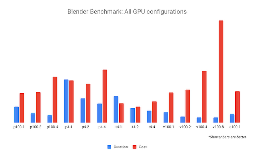
The NVIDIA V100-8 configuration may complete the benchmark fastest, but it also incurs the highest cost. The GPU configuration with the highest value appears to be 2x NVIDIA T4 GPUs, which complete the work fast enough to cost less than the 1x NVIDIA T4 GPU.
Finally, we compare all CPU and GPU configurations. The Blender Benchmark returns a duration, not a score, so we can use the cost of each benchmark to represent CPI. In the graph below, we use the n1-standard-8 (with a CPI of 1.0) as our target resource, to which we compare all other configurations:
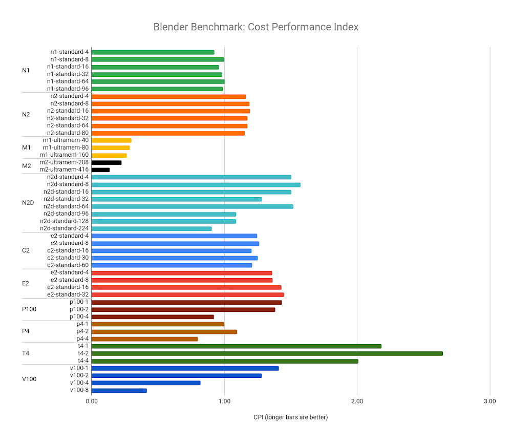
This confirms that the highest value configuration to run the Blender Benchmark is the 2x NVIDIA T4 GPU configuration running the benchmark in GPU mode.
Diminishing returns
Rendering on multiple GPUs can be more cost-effective than on a single GPU. The performance boost some renderers can gain from multiple GPUs can exceed that of the cost increase, which is linear.
The performance gains start to diminish as we add multiple V100s, therefore the value is also diminished when you factor in the increased cost. This observed flattening of the performance curve is an example of Amdahl’s Law. Adding resources to scale performance can result in a performance increase, but only up to a point, after which you tend to experience diminishing returns in performance. Many renderers are not capable of 100% parallelization, and therefore cannot scale linearly as resources are added.
As with GPU resources, the same can be observed across CPU resources. In this diagram, we observe how benchmark performance gains diminish as the number of N2D vCPUs climbs:
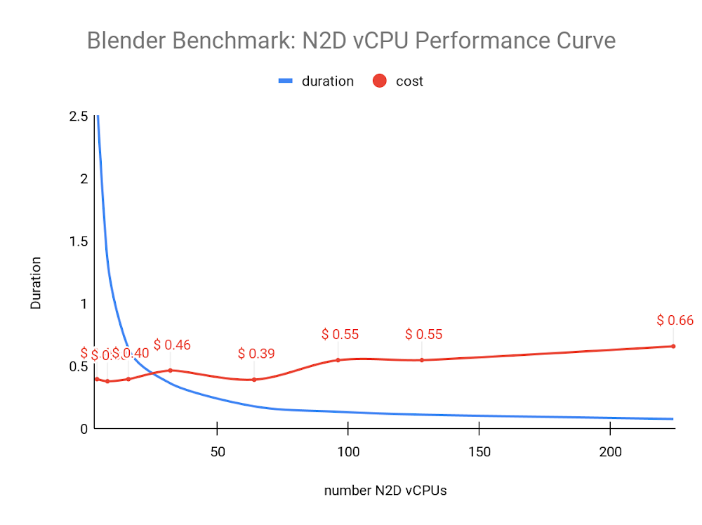
The above diagram shows that performance gains start to diminish above 64 vCPUs where the cost, surprisingly, drops a bit before climbing again.
Running the benchmarks
To ensure accurate, repeatable results, we built a simple, programmatic, reproducible testing framework that uses simple components of Google Cloud. We could also have used an established benchmarking framework such as PerfKit Benchmarker.
To observe the raw performance of each configuration, we ran each benchmark on a new instance running Ubuntu 1804. We ran each benchmark configuration six times in a row, discarding the first pass to account for local disk caching or asset load, and averaged the results of the remaining passes. This method, of course, doesn’t necessarily reflect the reality of a production environment where things like network traffic, queue management load, and asset synchronization may need to be taken into consideration.
Our benchmark workflow resembled the following diagram:

Examining the benchmarks
The renderers we benchmarked all have unique qualities, features, and limitations. Benchmark results revealed some interesting data, some of which is unique to a particular renderer or configuration, and some of which we found to be common across all rendering software.
Blender benchmark
Blender Benchmark was the most extensively tested of the benchmarks we ran. Blender’s renderer (called Cycles) is the only renderer in our tests that is able to run the same benchmark on both CPU and GPU configurations, allowing us to compare the performance of completely different architectures.
Blender Benchmark is freely available and is open source so you can even modify the code to include your own settings or render scenes.
The Blender Benchmark includes a number of different scenes to render. All our Blender benchmarks rendered the following scenes:
- bmw27
- classroom
- fishy_cat
- koro
- pavillon_barcelona
You can learn more about the above scenes on the Blender Demo Files page.
Download Blender Benchmark (version 2.90 used for this article)
Blender Benchmark documentation
Blender Benchmark public results
Benchmark observations
Blender Cycles appears to perform in a consistent fashion as resources are increased across all CPU and GPU configurations, although some configurations are subject to diminishing returns, as noted earlier:
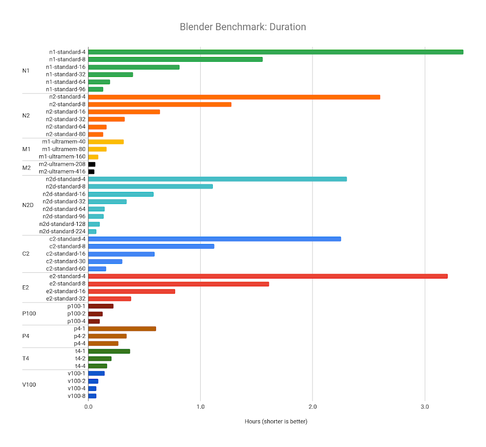
Next, we examine cost. With a few exceptions, all benchmarks cost between $0.40 and $0.60, no matter how many vCPUs or GPUs were used:
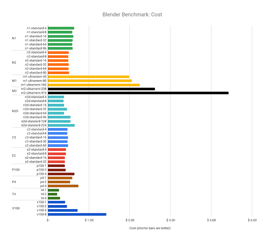
This may be more of a testament to how Google Cloud designed its resource cost model, but it’s interesting to note that each benchmark performed the exact same amount of work and generated the exact same output. Investigating the design of Blender Cycles and how it manages resource usage is beyond the scope of this article, however the source code is freely available for anyone to see, should they be interested in learning more.
The CPI of Blender is the inverse of the benchmark cost, but comparing it to our target resource (the n1-standard-8) reveals the highest value configurations to be any combination of T4 GPUs. The lowest value resources are the M2 machine types, due to their cost premium and the diminishing performance returns we see in the larger vCPU configurations:

V-Ray benchmark
V-Ray is a flexible renderer by ChaosGroup that is compatible with many 2D and 3D applications, as well as real time game engines.
V-Ray Benchmark is available as a standalone product for free (account registration required) and runs on Windows, Mac OS, and Linux. V-Ray can render in CPU and GPU modes, and even has a hybrid mode where it uses both.
V-Ray may run on both CPU and GPU, but their benchmarking software renders different sample scenes, and uses different units to compare results on each platform (CPU uses vsamples, GPU uses vpaths). We have grouped our V-Ray benchmark results into separate CPU and GPU configurations.
Download V-Ray Benchmark (version 5.00.01 used for this article)
V-Ray Bench documentation
V-Ray Bench public results
Benchmark observations
For CPU renders (using mode=vray for the benchmark), V-Ray appears to scale well as the number of vCPUs increases, and can take good advantage of the more modern CPU architectures offered on GCP, particularly the AMD EPYC in the N2D and the Intel Cascade Lake in the M2 Ultramem machine types:
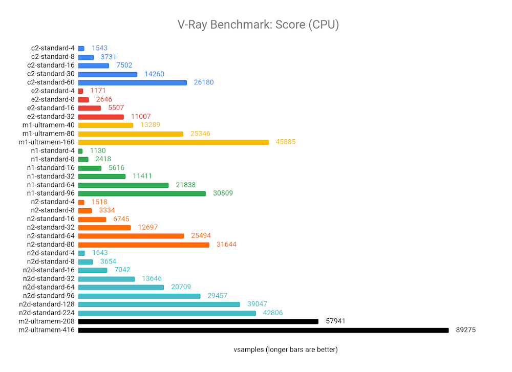
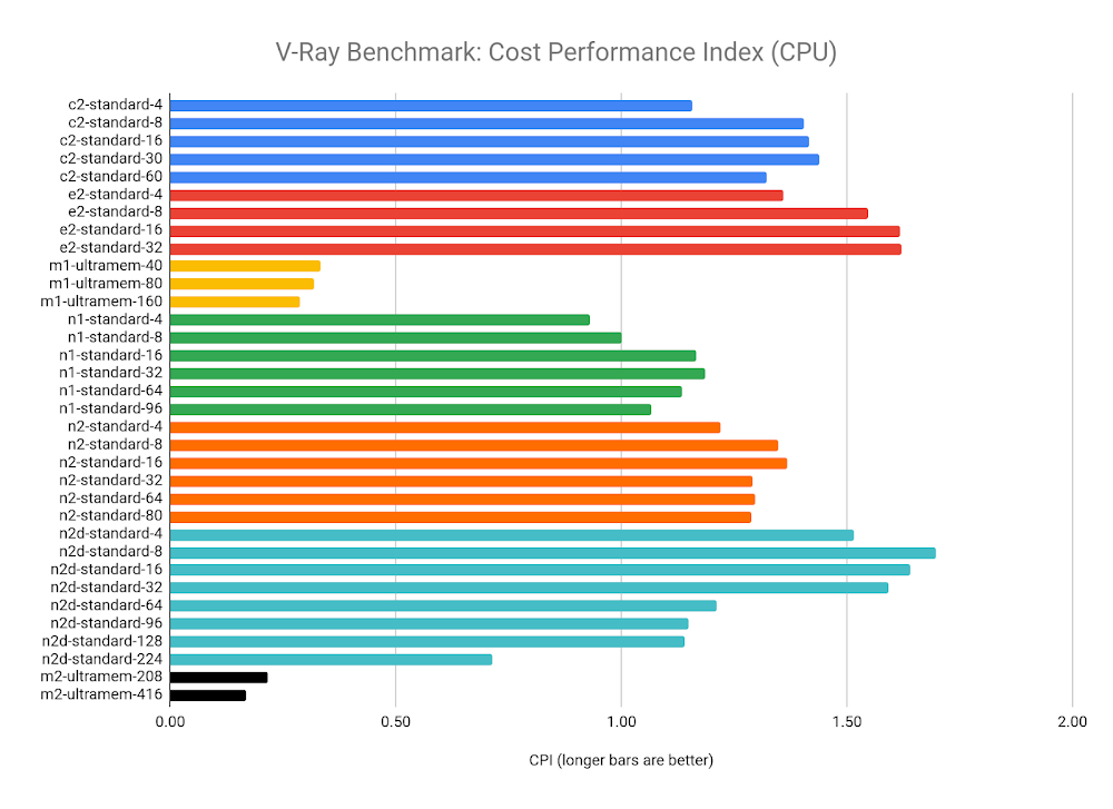
Looking at the CPI results, there appears to be a sweet spot where you get the most value out of V-Ray, somewhere between 8 and 64 vCPUs. Scores for 4 vCPU configurations all tend to be lower than the average of each machine type, and the larger configurations start to see diminishing returns as the vCPU count climbs.
The M1 and M2 Ultramem configurations are well below the CPI of our target resource (the n1-standard-8) as they have a cost premium that offsets their impressive performance. If you have the budget, however, you will get the best raw performance out of these machine types.
The best value appears to be from the N2D-standard-8, if your workload can fit into 32 GB of RAM:
In GPU mode (using mode=vray-gpu-cuda), V-Ray supports multiple GPUs well, scaling in a near-linear fashion with the number of GPUs.
It also appears that V-Ray is able to take good advantage of the new Ampere architecture on the A100 GPUs, showing a 30-35% boost in performance over the V100:
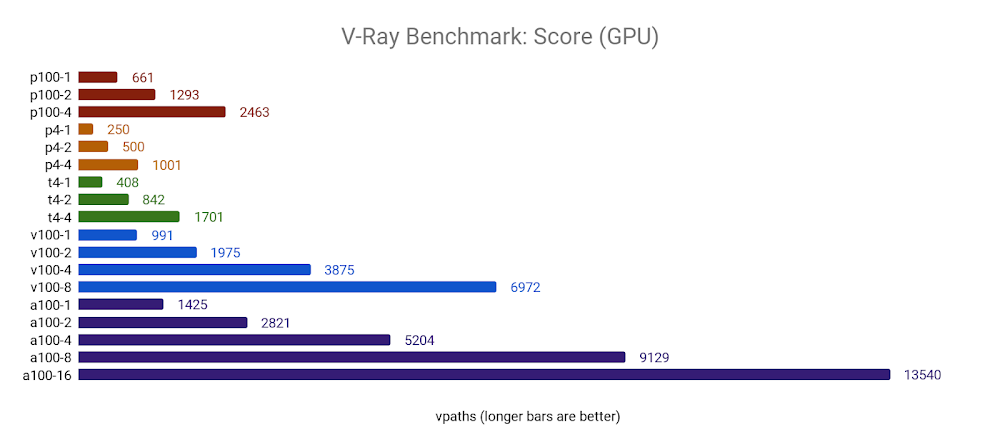
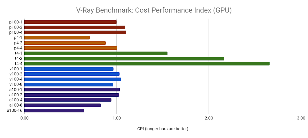
This boosted performance comes at a cost, however. The CPI for the 1x and 2xA100 configurations are only slightly better than the target resource (1xP100), and the 4x, 8x, and 16x configurations get increasingly expensive compared to performance capabilities.
As with all the other benchmarks, all configurations of the T4 GPU revealed the highest value GPU in the fleet:
Octane bench
Octane Render by OTOY is an unbiased, GPU-only renderer that is integrated with most popular 2D, 3D, and game engine applications.
Octane Bench is freely available for download and returns a score based on the performance of your configuration. Scores are measured in Ms/s (mega samples per second), and are relative to the performance of OTOY’s chosen baseline GPU, the NVIDIA GTX 980. See Octane Bench’s results page for more information on how the Octane Bench score is calculated.
Download Octane Bench (version 2020.1.4 used for this article)
Octane Bench documentation
Octane Bench public results
Benchmark observations
Octane Render scores relatively high across most GPUs offered on GCP, especially the a2-megagpu-16g machine type, which took the top score in their results when first publicly announced:
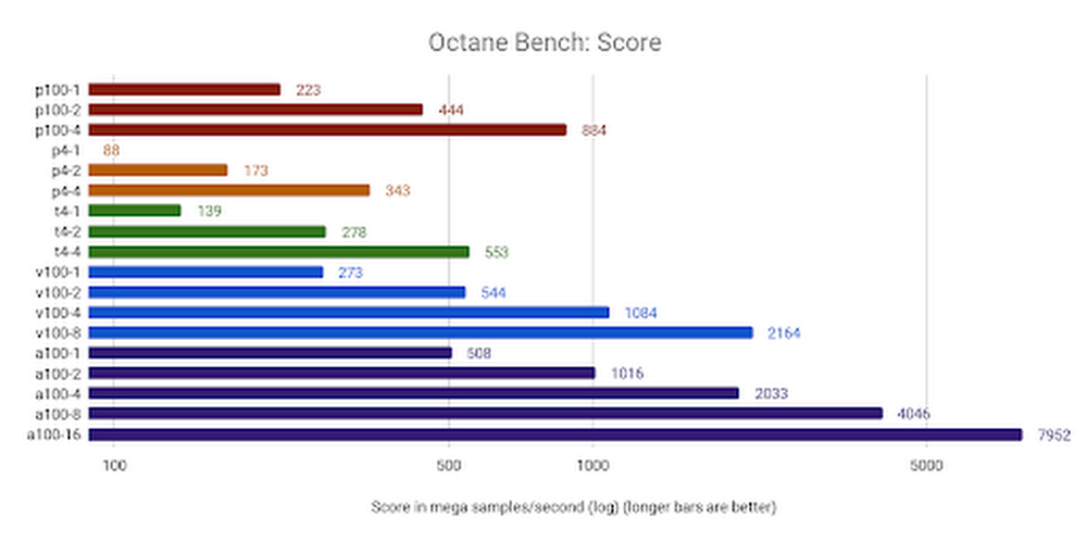
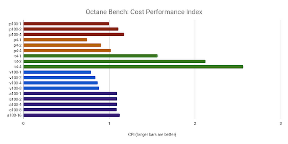
All configurations of the T4 delivered the most value, but P100’s and A100’s scored above the target resource. Interestingly, adding multiple GPUs improved the CPI in all cases, which is not always the case with the other benchmarks:
Redshift render
Redshift Render is a GPU-accelerated, biased renderer by Maxon, and integrates with 3D applications such as Maya, 3DS Max, Cinema 4D, Houdini, and Katana.
Redshift includes a benchmarking tool as part of the installation, and the demo version does not require a license to run the benchmark. To access the resources below, sign up for a free account here.
Download Redshift (version 3.0.31 used for this article)
Redshift Benchmark documentation
Redshift Benchmark public results
Benchmark observations
Redshift Render appears to scale in a linear manner as the number of GPUs is increased:
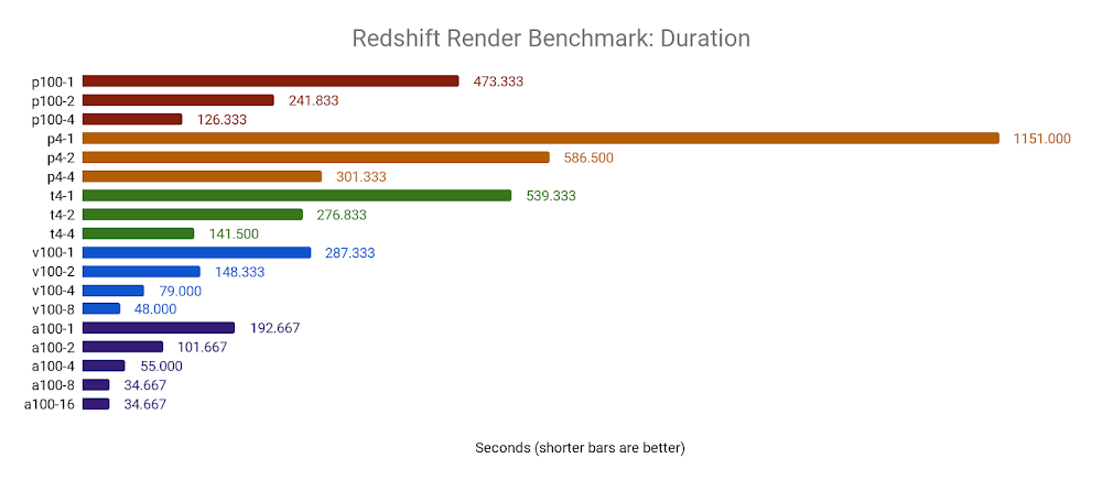
When benchmarking on the NVIDIA A100 GPUs, we start to see some limitations. Both the 8xA100 and 16xA100 configurations deliver the same results, and are only marginally faster than the 4xA100 configuration. Such a fast benchmark may be pushing the boundaries of the software itself, or may be limited by other factors such as the write performance of the attached persistent disk:
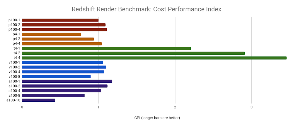
The NVIDIA T4 GPUs have the highest CPI by far, due to their low cost and competitive compute performance, particularly when multiple GPUs are used. Unfortunately, the limitations noted in the 8x and 16xA100 GPUs result in a lower CPI, but this could be due to the limits of this benchmark architecture and example scene.
Takeaways
This data can help customers who run rendering workloads decide which resources to use based on their individual job requirements, budget, and deadline. Some simple takeaways from this research:
If you aren’t time-constrained, and your render jobs don’t require lots of memory, you may want to choose smaller, preemptible configurations with higher CPI, such as the N2D or E2 machine types.
If you’re under a deadline and less concerned about cost, the M1 or M2 machine types (for CPU) or A2 machine types (for GPU) can deliver the highest performance, but may not be available as preemptible or may not be available in your chosen region.
Conclusion
We hope this research helps you better understand the characteristics of each compute platform and how performance and cost can be related for compute workloads.
Here are some final observations from all the render benchmarks we ran:
- For CPU renders, N2D machine types appear to provide the best performance at a reasonable cost, with the greatest flexibility (up to 224 vCPUs on a single VM).
- For GPU renders, the NVIDIA T4 delivers the most value due to its low price and Turing architecture, which is capable of running both RTX and TensorFlow workloads. You may not be able to run some larger jobs on the T4 however, as each GPU is limited to 16 GB of memory. If you need more GPU memory, you may want to look at a GPU type that offers NVLink, which unifies the memory of all attached GPUs.
- For sheer horsepower, the M2 machine types offer massive core counts (up to 416 vCPUs running at 4.0 GHz) with an astounding amount of memory (up to 11.7 GB). This may be overkill for most jobs, but a fluid simulation in Houdini or a 16k architectural render may need the extra resources to successfully complete.
- If you are in a deadline crunch or need to address last-minute changes, you can use the CPI of various configurations to help you cost model production workloads. When combined with performance metrics, you can accurately estimate how much a job should cost, how long it will take, and how well it will scale on a given architecture.
- The A100 GPUs in the A2 machine type offer massive gains over previous NVIDIA GPU generations, but we weren’t able to run all benchmarks on all configurations. The Ampere platform was relatively new when we ran our tests, and support for Ampere hadn’t been released for all GPU-capable rendering software.
Some customers choose resources based on the demands of their job, regardless of value. For example, a GPU render may require an unusually high amount of texture memory, and may only successfully complete on a GPU type that offers NVLink. In another scenario, a render job may have to be delivered in a short amount of time, regardless of cost. Both of these scenarios may steer the user towards the configuration that will get the job done, rather than the one with the highest CPI.
No two rendering workloads are the same, and no single benchmark can provide the true compute requirements for any job. You may want to run your own proof-of-concept render test to gauge how your own software, plugins, settings, and scene data perform on cloud compute resources.
Other benchmarking resources
Bear in mind we didn’t benchmark other metrics such as disk, memory, or network performance. See the following articles for more information, or to learn how to run your own benchmarks on Google Cloud:
Read More for the details.
