Today, Amazon SageMaker and Amazon DataZone announced a new data governance capability that enables customers to move a project from one domain unit to another. Domain units enable customers to create business unit/team level organization and manage authorization policies per their business needs. Customers can now take a project mapped to a domain unit and organize it under a new domain unit within their domain unit hierarchy. The move project feature lets customers reflect changes in team structures as business initiatives or organizations shift by allowing them to change a project’s owning domain unit.
As an Amazon SageMaker or Amazon DataZone administrator, you can now create domain units (e.g Sales, Marketing) under the top-level domain and organize the catalog by moving existing projects to new owning domain units. Users can then login to the portal to browse and search assets in the catalog by the domain units associated with their business units or teams.
The move project feature for domain units is available in all AWS Regions where Amazon SageMaker and Amazon DataZone are available.
Amazon Data Lifecycle Manager now offers customers the option to use Internet Protocol version 6 (IPv6) addresses for their new and existing endpoints. Customers moving to IPv6 can simplify their networks stack by running their Data Lifecycle Manager dual-stack endpoints on a network supporting both IPv4 and IPv6, depending on the protocol used by their network and client.
Customers create Amazon Data Lifecycle Manager policies to automate the creation, retention, and management of EBS Snapshots and EBS-backed Amazon Machine Images (AMIs). The policies can also automatically copy created resources across AWS Regions, move EBS Snapshots to EBS Snapshots Archive tier, and manage Fast Snapshot Restore. Customers can also create policies to automate creation and retention of application-consistent EBS Snapshots via pre and post-scripts, as well as create Default Policies for comprehensive protection for their account or AWS Organization.
Amazon Data Lifecycle Manager with IPv6, supported in all AWS Commercial Regions, is now available in the AWS GovCloud (US) Regions.
To learn more about configuring Amazon Data Lifecycle Manager endpoints for IPv6, please refer to our documentation.
AWS CodePipeline now supports Deploy Spec file configurations in the EC2 Deploy action, enabling you to specify deployment parameters directly in your source repository. You can now include either a Deploy Spec file name or deploy configurations in your EC2 Deploy action. The action accepts Deploy Spec files in YAML format and maintains compatibility with existing CodeDeploy AppSpec files.
The deployment debugging experience for large-scale EC2 deployments is also enhanced. Previously, customers relied solely on action execution logs to track deployment status across multiple instances. While these logs provide comprehensive deployment details, tracking specific instance statuses in large deployments was challenging. The new deployment monitoring interface displays real-time status information for individual EC2 instances, eliminating the need to search through extensive logs to identify failed instances. This improvement streamlines troubleshooting for deployments targeting multiple EC2 instances.
To learn more about how to use the EC2 deploy action, visit our documentation. For more information about AWS CodePipeline, visit our product page. These new actions are available in all regions where AWS CodePipeline is supported, except the AWS GovCloud (US) Regions and the China Regions.
AWS CodePipeline now offers a new Lambda deploy action that simplifies application deployment to AWS Lambda. This feature enables seamless publishing of Lambda function revisions and supports multiple traffic-shifting strategies for safer releases.
For production workloads, you can now deploy software updates with confidence using either linear or canary deployment patterns. The new action integrates with CloudWatch alarms for automated rollback protection – if your specified alarms trigger during traffic shifting, the system automatically rolls back changes to minimize impact.
To learn more about using this Lambda Deploy action in your pipeline, visit our documentation. For more information about AWS CodePipeline, visit our product page. These new actions are available in all regions where AWS CodePipeline is supported, except the AWS GovCloud (US) Regions and the China Regions.
Today, we’re excited to announce the general availability (GA) of GKE Data Cache, a powerful new solution for Google Kubernetes Engine to accelerate the performance of read-heavy stateful or stateless applications that rely on persistent storage via network attached disks. By intelligently utilizing high-speed local SSDs as a cache layer for persistent disks, GKE Data Cache helps you achieve lower read latency and higher queries per second (QPS), without complex manual configuration.
Using GKE Data Cache with Postgres we have seen:
Up to a 480% increase in transactions per second for PostgreSQL on GKE
Up to a 80% latency reduction for PostgreSQL on GKE
“The launch of GKE Persistent Disk with Data Cache enables significant improvements in vector search performance. Specifically, we’ve observed that Qdrant search response times are a remarkable 10x faster compared to balanced disks, and 2.5x faster compared to premium SSDs, particularly when operating directly from disk without caching all data and indexes in RAM. Qdrant Hybrid Cloud users on Google Cloud can leverage this advancement to efficiently handle massive datasets, delivering unmatched scalability and speed without relying on full in-memory caching.” – Bastian Hofmann, Director of Engineering, Qdrant
Stateful applications like databases, analytics platforms, and content management systems are critical to many businesses. However, their performance can often be limited by the I/O speed of the underlying storage. While persistent disks provide durability and flexibility, read-intensive workloads can experience bottlenecks, impacting application responsiveness and scalability.
GKE Data Cache addresses this challenge head-on, providing a managed block storage solution that integrates with your existing Persistent Disk or Hyperdisk volumes. When you enable GKE Data Cache on your node pools and configure your workloads to use it, frequently accessed data is automatically cached on the low-latency local SSDs attached to your GKE nodes.
This caching layer serves read requests directly from the local SSDs whenever the data is available, significantly reducing the need to access the underlying persistent disk and potentially allowing for the use of less system memory cache (RAM) to service requests in a timely manner.
aside_block
<ListValue: [StructValue([(‘title’, ‘$300 in free credit to try Google Cloud containers and Kubernetes’), (‘body’, <wagtail.rich_text.RichText object at 0x3e5757cc7130>), (‘btn_text’, ‘Start building for free’), (‘href’, ‘http://console.cloud.google.com/freetrial?redirectpath=/marketplace/product/google/container.googleapis.com’), (‘image’, None)])]>
The result is a substantial improvement in read performance, leading to:
Lower read latency: Applications experience faster data retrieval, improving the user experience and application responsiveness.
Higher throughput and QPS: The ability to serve more read requests in parallel allows your applications to handle increased load and perform more intensive data operations.
Potential cost optimization: By accelerating reads, you may be able to utilize smaller or lower-IOPS persistent disks for your primary storage while still achieving high performance through the cache. Additionally you may be able to reduce the required memory of the machine’s paging cache by pushing the read latency to the local SSD. Memory capacity is more expensive than capacity on a local SSD.
Simplified management: As a managed feature, GKE Data Cache simplifies the process of implementing and managing a high-performance caching solution for your stateful workloads.
“Nothing elevates developer experience like an instant feedback loop. Thanks to GKE Data Cache, developers can spin up pre-warmed Coder Workspaces on demand, blending local-speed coding with the consistency of ephemeral Kubernetes infrastructure.” – Ben Potter, VP of Product, Coder
GKE Data Cache supports all read/write Persistent Disk and Hyperdisk types as backing storage, so you can choose the right persistent storage for your needs while leveraging the performance benefits of local SSDs for reads. You can configure your node pools to dedicate a specific amount of local SSD space for data caching.
For data consistency, GKE Data Cache offers two write modes: writethrough (recommended for most production workloads to ensure data is written to both the cache and the persistent disk synchronously) and writeback (for workloads prioritizing write speed, with data written to the persistent disk asynchronously).
Getting started
Getting started with GKE Data Cache is straightforward. You’ll need a GKE Standard cluster running a compatible version (1.32.3-gke.1440000 or later), node pools configured with local SSDs, the data cache feature enabled, and a StorageClass that specifies the use of data cache acceleration. Your stateful workloads can then request storage with caching using PersistentVolumeClaims that reference this StorageClass. The amount of data to store in a cache for each disk is defined in the StorageClass.
Here’s how to create a data cache-enabled node pool in an existing cluster:
When you create a node pool with the `data-cache-count` flag, local SSDs (LSSDs) are reserved for the data cache feature. This feature uses those LSSDs to cache data for all pods that have caching enabled and are scheduled onto that node pool.
The LSSDs not reserved for caching can be used as ephemeral storage. Note that we do not currently support using the remaining LSSDs as raw block storage.
Once you reserve the required local SSDs for caching, you set up the cache configuration in the StorageClass with `data-cache-mode` and `data-cache-size` then reference that StorageClass in a PersistentVolumeClaim.
Building cutting-edge AI models is exciting, whether you’re iterating in your notebook or orchestrating large clusters. However, scaling up training can present significant challenges, including navigating complex infrastructure, configuring software and dependencies across numerous instances, and pinpointing performance bottlenecks.
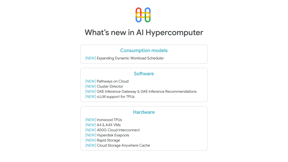
At Google Cloud, we’re focused on making AI training easier, whatever your scale. We’re continuously evolving our AI Hypercomputer system, not just with powerful hardware like TPUs and GPUs, but with a suite of tools and features designed to make you, the developer, more productive. Let’s dive into some recent enhancements that can help streamline your workflows, from interactive development to optimized training and easier deployment.
Scale from your notebook with Pathways on Cloud
You love the rapid iteration that Jupyter notebooks provide, but scaling to thousands of accelerators means leaving that familiar environment behind. At the same time, having to learn different tools for running workloads at scale isn’t practical; nor is tying up large clusters of accelerators for weeks for iterative experiments that might run only for a short time.
You shouldn’t have to choose between ease-of-use and massive scale. With JAX, it’s easy to write code for one accelerator and scale it up to thousands of accelerators. Pathways on Cloud, an orchestration system for creating large-scale, multi-task, and sparsely activated machine learning systems, takes this concept further, making interactive supercomputinga reality. Pathways dynamically manages pools of accelerators for you, orchestrating data movement and computation across potentially thousands of devices. The result? You can launch an experiment on just one accelerator directly from your Jupyter notebook, refine it, and then scale it to thousands of accelerators within the same interactive session. Now you can quickly iterate on research and development without sacrificing scale.
With Pathways on Cloud, you can finally stop rewriting code for different scales. Stop over-provisioning hardware for weeks when your experiments only need a few hours. Stay focused on your science, iterate faster, and leverage supercomputing power on demand. Watch this video to see how Pathways on Cloud delivers true interactive scaling — far beyond just running JupyterHub on a Google Kubernetes Engine (GKE) cluster.
When scaling up a job, simply knowing that your accelerators are being used isn’t enough. You need to understand how they’re being used and why things might be slow or crashing. How else would you find that pesky out-of-memory error that takes down your entire run?
Meet the Xprofiler library, your tool for deep performance analysis on Google Cloud accelerators. It lets you profile and trace your code execution, giving you critical insights, especially into the high level operations (HLO) generated by the XLA compiler. Getting actionable insights using Xprofiler is easy. Simply launch an Xprofiler instance from the command line to capture detailed profile and trace logs during your run. Then, use TensorBoard to quickly analyze this data. You can visualize performance bottlenecks, understand hardware limits with roofline analysis (is your workload compute- or memory-bound?), and quickly pinpoint the root cause of errors. Xprofiler helps you optimize your code for peak performance, so you can get the most out of your AI infrastructure.
Skip the setup hassle with container images
You have the choice of many powerful AI frameworks and libraries, but configuring them correctly — with the right drivers and dependencies — can be complex and time-consuming. Getting it wrong, especially when scaling to hundreds or thousands of instances, can lead to costly errors and delays. To help you bypass these headaches, we provide pre-built, optimized container images designed for common AI development needs.
For PyTorch on GPUs, our GPU-accelerated instance container images offer a ready-to-run environment. We partnered closely with NVIDIA to include tested versions of essential software like the NVIDIA CUDA Toolkit, NCCL, and frameworks such as NVIDIA NeMo. Thanks to Canonical, these run on optimized Ubuntu LTS. Now you can get started quickly with a stable environment that’s tuned for performance, avoiding compatibility challenges and saving significant setup time.
And if you’re working with JAX (on either TPUs or GPUs), our curated container images and recipes for JAX for AI on Google Cloud streamline getting started. Avoid the hassle of manual dependency tracking and configuration with these tested and ready-to-use JAX environments.
aside_block
<ListValue: [StructValue([(‘title’, ‘$300 in free credit to try Google Cloud infrastructure’), (‘body’, <wagtail.rich_text.RichText object at 0x3e575816a130>), (‘btn_text’, ‘Start building for free’), (‘href’, ‘http://console.cloud.google.com/freetrial?redirectPath=/compute’), (‘image’, None)])]>
Boost GPU training efficiency with proven recipes
Beyond setup, maximizing useful compute time (“ML Goodput”) during training is crucial, especially at scale. Wasted cycles due to job failures can significantly inflate costs and delay results. To help, we provide techniques and ready-to-use recipes to tackle these challenges.
Techniques like asynchronous and multi-tier checkpointing increase checkpoint frequency without slowing down training and speed up save/restore operations. AI Hypercomputer can automatically handle interruptions, choosing intelligently between resets, hot-swaps, or scaling actions. Our ML Goodput recipe, created in partnership with NVIDIA, bundles these techniques, integrating NVIDIA NeMo and the NVIDIA Resiliency Extension (NVRx) for a comprehensive solution to boost the efficiency and reliability of your PyTorch training on Google Cloud.
We also added optimized recipes (complete with checkpointing) for you to benchmark training performance for different storage options like Google Cloud Storage and Parallelstore. Lastly, we added recipes for our A4 NVIDIA accelerated instance (built on NVIDIA Blackwell). The training recipes include sparse and dense model training up to 512 Blackwell GPUs with PyTorch and JAX.
Cutting-edge JAX LLM development with MaxText
For developers who use JAX for LLMs on Google Cloud, MaxText provides advanced training, tuning, and serving on both TPUs and GPUs. Recently, we added support for key fine-tuning techniques like Supervised Fine Tuning (SFT) and Direct Preference Optimization (DPO), alongside resilient training capabilities such as suspend-resume and elastic training. MaxText leverages JAX optimizations and pipeline parallelism techniques that we developed in collaboration with NVIDIA to improve training efficiency across tens of thousands of NVIDIA GPUs. And we also added support and recipes for the latest open models: Gemma 3, Llama 4 training and inference (Scout and Maverick), and DeepSeek v3 training and inference.
To help you get the best performance with Trillium TPU, we added microbenchmarking recipes including matrix multiplication, collective compute, and high-bandwidth memory (HBM) tests scaling up to multiple slices with hundreds of accelerators. These metrics are particularly useful for performance optimization. For production workloads on GKE, be sure to take a look at automatic application monitoring.
Harness PyTorch on TPU with PyTorch/XLA 2.7 and torchprime
We’re committed to providing an integrated, high-performance experience for PyTorch users on TPUs. To that end, the recently released PyTorch/XLA 2.7 includes notable performance improvements, particularly benefiting users working with vLLM on TPU for inference. This version also adds an important new flexibility and interoperability capability: you can now call JAX functions directly from within your PyTorch/XLA code.
Then, to help you harness the power of PyTorch/XLA on TPUs, we introduced torchprime, a reference implementation for training PyTorch models on TPUs. Torchprime is designed to showcase best practices for large-scale, high-performance model training, making it a great starting point for your PyTorch/XLA development journey.
Build cutting-edge recommenders with RecML
While generative AI often captures the spotlight, highly effective recommender systems remain a cornerstone of many applications, and TPUs offer unique advantages for training them at scale. Deep-learning recommender models frequently rely on massive embedding tables to represent users, items, and their features, and processing these embeddings efficiently is crucial. This is where TPUs shine, particularly with SparseCore, a specialized integrated dataflow processor. SparseCore is purpose-built to accelerate the lookup and processing of the vast, sparse embeddings that are typical in recommenders, dramatically speeding up training compared to alternatives.
To help you leverage this power, we now offer RecML: an easy-to-use, high-performance, large-scale deep-learning recommender system library optimized for TPUs. It provides reference implementations for training state-of-the-art recommender models such as BERT4Rec, Mamba4Rec, SASRec, and HSTU. RecML uses SparseCore to maximize performance, making it easy for you to efficiently utilize the TPU hardware for faster training and scaling of your recommender models.
Build with us!
Improving the AI developer experience on Google Cloud is an ongoing mission. From scaling your interactive experiments with Pathways, to pinpointing bottlenecks with Xprof, to getting started faster with optimized containers and framework recipes, these AI Hypercomputer improvements help to remove friction so you can innovate faster, and build on the other AI Hypercomputer innovations we announced at Google Cloud Next 25:
Explore these new features, spin up the container images, try the JAX and PyTorch recipes, and contribute back to open-source projects like MaxText, torchprime, and RecML. Your feedback shapes the future of AI development on Google Cloud. Let’s build it together.
Organizations depend on fast and accurate data-driven insights to make decisions, and SQL is at the core of how they access that data. With Gemini, Google can generate SQL directly from natural language — a.k.a. text-to-SQL. This capability increases developer and analysts’ productivity and empowers non-technical users to interact directly with the data they need.
Today, you can find text-to-SQL capabilities in many Google Cloud products:
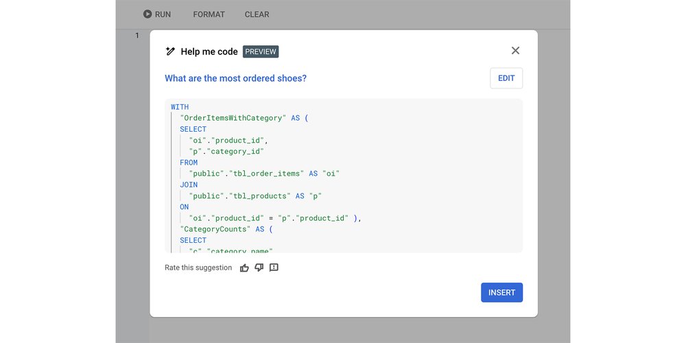
“Help me code” functionality in Cloud SQL Studio (Postgres, MySQL and SQLServer), AlloyDB Studio and Cloud Spanner Studio
AlloyDB AI with its direct natural language interface to the database, currently available as a public preview
Through Vertex AI, which lets you access the Gemini models that are the basis for these products directly
Recently, powerful large language models (LLMs) like Gemini, with their abilities to reason and synthesize, have driven remarkable advancements in the field of text-to-SQL. In this blog post, the first entry in a series, we explore the technical internals of Google Cloud’s text-to-SQL agents. We will cover state-of-the-art approaches to context building and table retrieval, how to do effective evaluation of text-to-SQL quality with LLM-as-a-judge techniques, the best approaches to LLM prompting and post-processing, and how we approach techniques that allows the system to offer virtually certified correct answers.
The ‘Help me code’ feature in Cloud SQL Studio generates SQL from a text prompt
The challenges of text-to-SQL technology
Current state-of-the-art LLMs like Gemini 2.5 have reasoning capabilities that make them good at translating complex questions posed in natural language to functioning SQL, complete with joins, filters, aggregations and other difficult concepts.
To see this in action you can do a simple test in Vertex AI Studio. Given the prompt “I have a database schema that contains products and orders. Write a SQL query that shows the number of orders for shoes”, Gemini produces SQL for a hypothetical schema:
code_block
<ListValue: [StructValue([(‘code’, “SELECT COUNT(DISTINCT o.order_id) AS NumberOfShoeOrders FROM orders o JOIN order_items oi ON o.order_id = oi.order_id JOIN products p ON oi.product_id = p.product_id WHERE p.product_name LIKE ‘%shoe%’.”), (‘language’, ”), (‘caption’, <wagtail.rich_text.RichText object at 0x3eaaccfde9d0>)])]>
Great, this is a good looking query. But what happens when you move beyond this trivial example, and use Gemini for text-to-SQL against a real world database and on real-world user questions? It turns out that the problem is more difficult. The model needs to be complemented with methods to:
provide business-specific context
understand user intent
manage differences in SQL dialects
Let’s take a look at each of these challenges.
Problem #1: Provide business-specific context
Just like data analysts or engineers, LLMs need significant amounts of knowledge or “context” to generate accurate SQL. The context can be both explicit (what does the schema look like, what are the relevant columns, and what does the data itself look like?) or more implicit (what is the precise semantic meaning of a piece of data? what does it mean for the specific business case?).
Specialized model training, or fine tuning, is typically not a scalable solution to this problem. Training on the shape of every database or dataset, and keeping up with schema or data changes, is both difficult and cost-prohibitive. Business knowledge and semantics are often not well documented in the first place, and difficult to turn into training data.
For example, even the best DBA in the world would not be able to write an accurate query to track shoe sales if they didn’t know that cat_id2 = 'Footwear' in a pcat_extension table means that the product in question is a kind of shoe. The same is true for LLMs.
Problem #2: Understanding user intent
Natural language is less precise than SQL. An engineer or analyst faced with an ambiguous question can detect that they need more information and go back and ask the right follow-up questions. An LLM, on the other hand, tends to try to give you an answer, and when the question is ambiguous, can be prone to hallucinating.
Example: Take a question like “What are the best-selling shoes?” Here, one obvious point of ambiguity is what “best selling” actually means in the context of the business or application — the most ordered shoes? The shoe brand that brought in the most money? Further, should the SQL count returned orders? And how many kinds of shoes do you want to see in the report? etc.
Further, different users need different kinds of answers. If the user is a technical analyst or a developer asking a vague question, giving them a reasonable, but perhaps not 100% correct SQL query is a good starting point. On the other hand, if the user is less technical and does not understand SQL, providing precise, correct SQL is more important. Being able to reply with follow-up questions to disambiguate, explaining the reasoning that went into an answer, and guiding the user to what they are looking for is key.
Problem #3: Limits of LLM generation
Out of the box, LLMs are particularly good at tasks like creative writing, summarizing or extracting information from documents. But some models can struggle with following precise instructions and getting details exactly right, particularly when it comes to more obscure SQL features. To be able to produce correct SQL, the LLM needs to adhere closely to what can often turn into complex specifications.
Example: Consider the differences between SQL dialects, which are more subtle than differences between programming languages like Python and Java. As a simple example, if you’re using BigQuery SQL, the correct function for extracting a month from a timestamp column is EXTRACT(MONTH FROM timestamp_column). But if you are using MySQL, you use MONTH(timestamp_column).
Text-to-SQL techniques
At Google Cloud, we’re constantly evolving our text-to-SQL agents to improve their quality. To address the problems listed above, we apply a number of techniques.
Problem
Solutions
Understanding schema, data and business concepts
Intelligent retrieval and ranking of datasets, tables and columns, based on semantic similarity.
In-context-learning with business specific examples
Data linking and sampling
Semantic layer over raw data. This provides a bridge between complex data structures and the everyday language used by the customer
Usage pattern analysis and query history
Understanding user intent
Disambiguation using LLMs
Entity resolution
SQL-aware foundation models
Limits of LLM generation
Self-consistency
Validation and rewriting
Strong foundation models
In-context-learning with dialect specific examples
Model finetuning
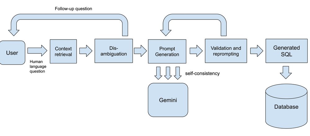
The text-to-SQL architecture
Let’s take a closer look at some of these techniques.
SQL-aware models Strong LLMs are the foundation of text-to-SQL solutions, and the Gemini family of models has a proven track record of high-quality code and SQL generation. Depending on the particular SQL generation task, we mix and match model versions, including some cases where we employ customized fine-tuning, for example to ensure that models provide sufficiently good SQL for certain dialects.
Disambiguation using LLMs Disambiguation involves getting the system to respond with a clarifying question when faced with a question that is not clear enough (in the example above of “What is the best selling shoe?” should lead to a follow-up question like “Would you like to see the shoes ordered by order quantity or revenue?” from the text-to-SQL agent). Here we typically orchestrate LLM calls to first try to identify if a question can actually be answered given the available schema and data, and if not, to generate the necessary follow-up questions to clarify the user’s intent.
Retrieval and in-context-learning As mentioned above, providing models with the context they need to generate SQL is critical. We use a variety of indexing and retrieval techniques — first to identify relevant datasets, tables and columns, typically using vector search for multi-stage semantic matching, then to load additional useful context. Depending on the product, this may include things like user-provided schema annotations, examples of similar SQL or how to apply specific business rules, or samples of recent queries that a user has run against the same datasets. All of this data is organized into prompts then passed to the model. Gemini’s support for long context windows unlocks new capabilities here by allowing the model to handle large schemas and other contextual information.
Validation and reprompting Even with a high-quality model, there is still some level of non-determinism or unpredictability involved in LLM-driven SQL generation. To address this we have found that non-AI approaches like query parsing or doing a dry run of the generated SQL complements model-based workflows well. We can get a clear, deterministic signal if the LLM has missed something crucial, which we then pass back to the model for a second pass. When provided an example of a mistake and some guidance, models can typically address what they got wrong.
Self-consistency The idea of self-consistency is to not depend on a single round of generation, but to generate multiple queries for the same user question, potentially using different prompting techniques or model variants, and picking the best one from all candidates. If several models agree that one answer looks particularly good, there is a greater chance that the final SQL query will be accurate and matches what the user is looking for.
Evaluation and measuring improvements
Improving AI-driven capabilities depends on robust evaluation. The text-to-SQL benchmarks developed in the academic community, like the popular BIRD-bench, have been a very useful baseline to understand model and end-to-end system performance. However, these benchmarks are often lacking when it comes to representing broad real-world schemas and workloads. To address this we have developed our own suite of synthetic benchmarks that augment the baseline in many ways.
Coverage: We make sure to have benchmarks that cover a broad list of SQL engines and products, both dialects and engine-specific features. This includes not only queries, but also DDL, DML and other administrative needs, and questions that are representative for common usage patterns, including more complex queries and schemas.
Metrics: We combine user metrics and offline eval metrics, and employ both human and automated evaluation, particularly using LLM-as-a-judge techniques, which reduce cost but still allow us to understand performance on ambiguous and unclear tasks.
Continuous evals: Our engineering and research teams use evals to quickly be able to test out new models, new prompting techniques and other improvements. It can give us signals quickly to tell if an approach is showing promise and is worth pursuing.
Taken together, using these techniques are driving the remarkable improvements in text-to-SQL that we are witnessing in our labs, as well as in customers’ environments. As you get ready to incorporate text-to-SQL in your own environments, stay tuned for more deep dives into our text-to-SQL solutions. Try Gemini text-to-SQL in BigQuery Studio, CloudSQL, AlloyDB and Spanner Studio, and in AlloyDB AI today.
We are pleased to announce that the memory allocation per OpenSearch Compute Unit (OCU) for Amazon OpenSearch Ingestion has been increased from 8GB to 15GB. One OCU now comes default with 2vCPU and 15GB of memory, allowing customers to leverage greater in-memory processing for their data ingestion pipelines without modifying existing configurations.
With the increased memory per OCU, Amazon OpenSearch Ingestion is better equipped to handle memory-intensive processing tasks such as trace analytics, aggregations, and enrichment operations. Customers can now build more complex and high-throughput ingestion pipelines with reduced risk of out-of-memory failures.
The increased memory for OCUs are now available in all AWS Regions where Amazon OpenSearch Ingestion is currently offered at no additional cost. You can take advantage of these improvements by updating your existing pipelines or creating new pipelines through the Amazon OpenSearch Service console or APIs at no additional cost.
Today, Simple Email Service (SES) Mail Manager announces the addition of a Debug logging level for Mail Manager traffic policies. This new logging level provides more detailed visibility on incoming connections to a customer’s Mail Manager ingress endpoint and makes it easier to troubleshoot delivery challenges quickly, using familiar event destinations such as Cloudwatch, Kinesis, and S3.
With Debug level logs, customers can now log every possible evaluation and action within a Mail Manager traffic policy, along with envelope data for the email message being evaluated for traffic permission. This enables customers to determine whether their traffic policy is working as expected or to isolate incoming message parameters which are not covered by the current configuration. When used in conjunction with rules engine logging, debug logging for traffic policies charts a full picture of message arrival into Mail Manager and its disposition by the rules engine. Debug logging for traffic policies is intended to be used during active troubleshooting but otherwise left disabled, as its output can be verbose for high-volume Mail Manager instances. While SES does not charge an additional fee for this logging feature, customers may incur costs from their chosen event destination.
Debug logging for traffic policies is available in all 17 AWS non-opt-in Regions within the AWS commercial partition. To learn more about Mail Manager logging options, see the SES Mail Manager Logging Guide.
AWS Parallel Computing Service (PCS) now supports Slurm version 24.11 with support for managed accounting. Using this feature, you can enable accounting on your PCS clusters to monitor cluster usage, enforce resource limits, and manage fine-grained access control to specific queues or compute node groups. PCS manages the accounting database for your cluster, eliminating the need for you to setup and manage a separate accounting database.
You can enable this feature on your PCS cluster in just a few clicks using the AWS Management Console. Visit our getting started and accounting documentation pages to learn more about accounting and see release notes to learn more about Slurm 24.11.
AWS Parallel Computing Service (AWS PCS) is a managed service that makes it easier for you to run and scale your high performance computing (HPC) workloads and build scientific and engineering models on AWS using Slurm. To learn more about PCS, refer to the service documentation. For pricing details and region availability, see the PCS Pricing Page and AWS Region Table.
AWS CodeBuild now supports remote Docker image build servers, allowing you to speed up image build requests. You can provision a fully managed Docker server that maintains a persistent cache across builds. AWS CodeBuild is a fully managed continuous integration service that compiles source code, runs tests, and produces ready-to-deploy software packages.
Centralized image building increases efficiency by reusing cached layers and reducing provisioning plus network transfer latency. CodeBuild automatically configures your build environment to use the remote server when running Docker commands. The Docker server is then readily available to run parallel build requests that can each use the shared layer cache, reducing the overall build latency and optimizing build speed.
This feature is available in all regions where CodeBuild is offered. For more information about the AWS Regions where CodeBuild is available, see the AWS Regions page.
Today’s businesses have a vital need to manage and, when appropriate, transfer cyber risk in their cloud environments — even with robust security measures in place. At Google Cloud Next last month, we unveiled significant advancements to our Risk Protection Program, an industry-first collaboration between Google and leading cyber insurers that provides competitively priced cyber-insurance and broad coverage for Google Cloud customers.
These updates make the program more accessible to more organizations, expand our specialized cyber insurance offerings, and can help increase your overall confidence in your ability to successfully manage the cyber risk your organization faces. The Risk Protection Program (RPP) is based on your cloud security posture as reported through Security Command Center (SCC), and reinforces our shared fate model as we actively partner with you for risk management.
New in 2025: Broader access, more choice
The Risk Protection Program has two main components:
Cyber Insurance Hub, provided by Google: This tool enables a quick assessment of your risk posture across Google Cloud and facilitates a streamlined process for procuring cyber insurance.
Tailored Cyber Insurance Policies, provided by partners: These are available through a modern, low-friction underwriting process, and use data submitted by customers to enable personalized pricing based on their specific use and risk posture.
To further enhance the value and accessibility of these core components, we’re introducing several key updates.
New insurance partners, expanded global reach
Giving Google Cloud customers a wider array of choices for tailored cyber insurance, we’re excited to welcome Beazley and Chubb, two of the world’s largest cyber-insurers, as new program partners. We are also expanding our collaboration with our founding partner, Munich Re, through onboarding Munich Re Specialty and their SMB-focused subsidiary HSB.
This collaboration will make the Risk Protection Program available to more Google Cloud customers, extending our reach to include businesses of all sizes. We’re also expanding the program’s availability internationally, with coverage rolling out in phases, ensuring that more organizations can take advantage of the unique benefits of the program.
Streamlined insurance procurement and data-driven pricing
The Cyber Insurance Hub can help you measure and manage your risk directly on Google Cloud. It assesses your Google Cloud workloads and provides proactive security recommendations. It also generates reports that map your cloud configurations against the industry-standard CIS Benchmarks.
The hub allows you to directly share your actual risk posture data — derived from your real-world cloud setup — with participating cyber insurers through a streamlined interface. This represents a significant improvement over traditional, often lengthy, and manual insurance applications, crafting a more efficient underwriting process that can deliver potentially more competitive and appropriate pricing.
aside_block
<ListValue: [StructValue([(‘title’, ‘$300 in free credit to try Google Cloud security products’), (‘body’, <wagtail.rich_text.RichText object at 0x3e25c569df10>), (‘btn_text’, ‘Start building for free’), (‘href’, ‘http://console.cloud.google.com/freetrial?redirectPath=/welcome’), (‘image’, None)])]>
Accelerated onboarding for digital natives
Additionally, for qualified Google Cloud digital native customers, Beazley is removing the traditional, often complex insurance application altogether and replacing it with a single-page attestation. This means an even faster, simpler path to securing tailored cyber insurance for organizations deeply integrated with Google Cloud.
Coverage for emerging AI risks
The Risk Protection Program is further evolving to address the rapidly changing technological landscape, including the increasing adoption of AI. A key enhancement now available is the inclusion of Affirmative AI insurance coverage for your Google-related AI workloads. Building upon Google’s existing AI indemnification commitment, this explicit coverage provides clarity and reduces uncertainty around the unique risks associated with generative AI.
Preparedness against future quantum threats
Demonstrating a commitment to future-forward risk management, Chubb’s offerings will include coverage specifically against potential future quantum exploit risks. This proactive step aligns with Google’s ongoing work in post-quantum cryptography (PQC) and helps customers prepare for potential security challenges posed by future quantum computing advancements.
Threat intelligence, advisory and incident preparedness with Mandiant
Risk Protection Program clients underwritten by Munich Re receive access to Mandiant’s expertise in threat intelligence, advisory, and incident preparedness.
This expertise includes near real-time updates on high-priority exploited vulnerabilities informed by Mandiant Consulting and Google Threat Intelligence Group, technical coaching from experienced Mandiant incident responders during a cybersecurity incident, and tabletop exercises facilitated by Munich Re and Mandiant Consulting to test and enhance incident readiness with your teams.
Translating security investments into financial returns
The enhanced Risk Protection Program helps translate your dedication to security into tangible business value. By using the Cyber Insurance Hub and demonstrating strong security practices on Google Cloud, you can potentially achieve more favorable terms and pricing on cyber insurance premiums — the return on investment is clear.
We understand that navigating the complexities of cloud risk can be new to some insurers, which is why Google actively works with our cyber insurance partners to ensure they understand the nuances of the cloud, simplifying the process for you.
“Google Cloud’s Risk Protection Program has streamlined our insurance underwriting process while providing valuable insight into quantitative risks through standardized reporting, enhanced compliance monitoring, and simplified reporting to our insurance provider. This partnership underscores our shared commitment to safeguarding trust and ensuring the responsible use of data,” said Frank Caserta, CISO, LiveRamp.
“We were early adopters of RPP and it’s been a great change in our process. The program has helped us have a more efficient renewal … I just go and I press one button and it goes off to insurance partners. Because I know what data the insurance underwriters are going to be using, I can proactively respond to any questions and therefore cut down time dramatically. To organizations looking to adopt RPP, I would say do it. It makes your insurance renewal process so much more efficient,” said Justinian Fortenberry, CISO and VP of Engineering, Etsy.
It’s easy to get started
At Google Cloud, we firmly believe that the cloud is more than just a risk to be managed, it is a platform for managing risk effectively. Our new enhancements to the Risk Protection Program mark a significant step forward in helping customers navigate the complexities of cloud security and risk management.
To get started, you can follow these four steps:
Discuss the Risk Protection Program with your insurance lead and broker.
Onboard to Google’s Cyber Insurance Hub, run a report, and share the report with your chosen insurance partner(s).
Work with your insurance broker to complete the cyber insurance underwriting process, and evaluate any quotes.
AWS Transform for .NET, previewed as “Amazon Q Developer transformation capabilities for .NET porting,” is now generally available. As the first agentic AI service for modernizing .NET applications at scale, AWS Transform helps you to modernize Windows .NET applications to be Linux-ready up to four times faster than traditional methods and realize up to 40% savings in licensing costs. It supports transforming a wide range of .NET project types including MVC, WCF, Web API, class libraries, console apps, and unit test projects.
The agentic transformation begins with a code assessment of your repositories from GitHub, GitLab, or Bitbucket. It identifies .NET versions, project types, and interproject dependencies and generates a tailored modernization plan. You can customize and prioritize the transformation sequence based on your business objectives or architectural complexity before initiating the AI-powered modernization process. Once started, AWS Transform for .NET automatically converts application code, builds the output, runs unit tests, and commits results to a new branch in your repository. It provides a comprehensive transformation summary, including modified files, test outcomes, and suggested fixes for any remaining work. Your teams can track transformation status through the AWS Transform dashboards or interactive chat and receive email notifications with links to transformed .NET code. For workloads that need further human input, your developers can continue refinement using the Visual Studio extension in AWS Transform. The scalable experience of AWS Transform enables consistent modernization across a large application portfolio while moving to cross-platform .NET, unlocking performance, portability, and long-term maintainability.
AWS Transform for .NET is now available in the following AWS Regions: US East (N. Virginia) and Europe (Frankfurt).
AWS Transform for mainframe, previewed as “Amazon Q Developer transformation capabilities for mainframe” at re:Invent 2024, is now generally available. AWS Transform is the first agentic AI service for modernizing mainframe applications at scale—accelerating modernization of IBM z/OS applications from years to months.
Powered by a specialized AI agent leveraging 19 years of AWS experience, AWS Transform streamlines the entire transformation process—from initial analysis and planning to code documentation and refactoring—helping organizations to modernize faster, reduce risk and cost, and achieve better outcomes in the cloud.
This release introduces significant new capabilities. Enhanced analysis features help teams identify cyclomatic complexity, homonyms, and duplicate IDs across codebases, with new export and import functions for file classification and in-UI file viewing and comparison. Documentation generation now supports larger codebases with improved performance and recovery capabilities, including an AI-powered chat experience for querying generated documentation.
Teams can use improved decomposition features to manage dependencies and domain creation, while new deployment templates streamline environment setup for modernized applications. The service also introduces flexible job management, allowing teams to modify objectives and focus on specific transformation steps during reruns.
AWS Transform for mainframe is available in the following AWS Regions: US East (N. Virginia) and Europe (Frankfurt).
Today, AWS announces the general availability of migration assessment capabilities in AWS Transform. Migration assessment in AWS Transform analyzes your IT environment to simplify and optimize your cloud journey with intelligent, data-driven insights and actionable recommendations. Simply upload your infrastructure data and AWS Transform will deliver a comprehensive analysis that typically takes weeks in just minutes.
Powered by agentic AI, AWS Transform removes weeks of manual analysis by providing instant visibility into your infrastructure and automatically discovering cost optimization opportunities. AWS Transform produces a business case including key highlights from your server inventory, a summary of current infrastructure, multiple TCO scenarios with varying purchase commitments (on-demand and reserved instances), operating system licensing options (bring your own licenses and license-included), and tenancy options.
AWS Transform for migration assessments is now available in the following AWS Regions: US East (N. Virginia) and Europe (Frankfurt).
Ready to get started? Visit the AWS Transform web experience or read our blog post to learn more.
At re:Invent 2024, AWS introduced the preview of Amazon Q Developer transformation capabilities for VMware. That innovation has evolved into AWS Transform for VMware—a first-of-its-kind agentic AI service that’s now generally available. Powered by large language models, graph neural networks, and the deep experience of AWS in enterprise workload migrations, AWS Transform simplifies VMware modernization at scale. Customers and partners can now move faster, reduce migration risk, and modernize with confidence.
VMware environments have long been foundational to enterprise IT, but rising costs and vendor uncertainty are prompting organizations to rethink their strategies. Despite the urgency, VMware workload migration has historically been slow and error-prone. AWS Transform changes that. With agentic AI, AWS Transform automates the full modernization lifecycle—from discovery and dependency mapping to network translation and Amazon Elastic Compute Cloud (Amazon EC2) optimization. Certain tasks that once took weeks can now be completed in minutes. In testing, AWS generated migration wave plans for 500 VMs in just 15 minutes and performed networking translations up to 80x faster than traditional methods. Partners in pilot programs have cut execution times by up to 90%.
Beyond speed, AWS Transform delivers precision and transparency. A shared workspace brings together infrastructure teams, app owners, partners, and AWS experts to resolve blockers and maintain alignment. Built-in human-in-the-loop controls confirm all artifacts are validated before execution. As enterprises aim to break free from legacy constraints and tap into the value of their data, AWS Transform offers a streamlined path to modern, cloud-native architectures. Customers can seamlessly integrate with 200+ AWS services—including analytics, serverless, and generative AI—to accelerate innovation and reduce long-term costs.
Amazon SageMaker Catalog integrates with Amazon S3 Tables, making it easy to discover, share, and govern S3 Tables for users to access and query the data with all Apache Iceberg–compatible tools and engines. With Amazon SageMaker Catalog, built on Amazon DataZone, users can securely discover and access approved data and models using semantic search with generative AI–created metadata, or just ask Amazon Q Developer with natural language to find your data.
S3 Tables deliver the first cloud object store with built-in Apache Iceberg support. Data publishers can onboard S3 tables to SageMaker Lakehouse and enhance their discoverability by adding them to the SageMaker Catalog. Publishers have the flexibility to either directly publish tables or enrich them with valuable business metadata, making it easier for all users to understand and find the data they need. On the consumption side, users can search for relevant tables, request access through a subscription workflow (subject to publisher approval), and leverage this data for advanced analytics and AI development projects. This end-to-end workflow significantly improves data accessibility, governance, and utilization of S3 Tables across the organization.
SageMaker Catalog with S3 Tables support is available in all AWS Regions where Amazon SageMaker is available.
Today, AWS Glue Studio announces support for additional compressed file types, Excel files (as source), and XML and Tableau’s Hyper files (as target). We are also introducing the option to select the number of output files for an S3 target. These enhancements will allow you to use visual ETL jobs for additional data processing workflows not supported today, for example loading data from an Excel file into a single XML file output.
The new experience will now enable you to have one single file as the output of your Glue job, or to specify a custom number for the output files. Further, Glue now supports Excel files via S3 file source nodes, and XML or Tableau Hyper files for S3 file target nodes. New compression types that will be available to use are: LZ4 , SNAPPY, DEFLATE, LZO, BROTLI, ZSTD and ZLIB.
These new features are now available in all AWS commercial Regions and AWS GovCloud (US) Regions where AWS Glue is available. Access the AWS Regional Services List for the most up-to-date availability information.
Amazon RDS for PostgreSQL 18 Beta 1 is now available in the Amazon RDS Database Preview Environment, allowing you to evaluate the pre-release of PostgreSQL 18 on Amazon RDS for PostgreSQL. You can deploy PostgreSQL 18 Beta 1 in the Amazon RDS Database Preview Environment that has the benefits of a fully managed database.
PostgreSQL 18 includes significant updates to query execution and I/O operations. Query execution is enhanced with “skip scan” support for multicolumn B-tree indexes and optimized WHERE clause handling for OR and IN (…) conditions. Parallel execution capabilities are expanded through parallel GIN index builds and enhanced join operations. Observability improvements include detailed buffer access statistics in EXPLAIN ANALYZE and enhanced I/O utilization monitoring capabilities. Please refer to the PostgreSQL community announcement for more details.
Amazon RDS Database Preview Environment database instances are retained for a maximum period of 60 days and are automatically deleted after the retention period. Amazon RDS database snapshots that are created in the preview environment can only be used to create or restore database instances within the preview environment. You can use the PostgreSQL dump and load functionality to import or export your databases from the preview environment.
Amazon RDS Database Preview Environment database instances are priced as per the pricing in the US East (Ohio) Region.
Today, AWS announces the general availability of Amazon Elastic Compute Cloud (Amazon EC2) P6-B200 instances, accelerated by NVIDIA B200 GPUs. Amazon EC2 P6-B200 instances offer up to 2x performance compared to P5en instances for AI training and inference.
P6-B200 instances feature 8 Blackwell GPUs with 1440 GB of high-bandwidth GPU memory and a 60% increase in GPU memory bandwidth compared to P5en, 5th Generation Intel Xeon processors (Emerald Rapids), and up to 3.2 terabits per second of Elastic Fabric Adapter (EFAv4) networking. P6-B200 instances are powered by the AWS Nitro System, so you can reliably and securely scale AI workloads within Amazon EC2 UltraClusters to tens of thousands of GPUs.