GCP – TimesFM in Data Cloud: The future of forecasting in BigQuery and AlloyDB
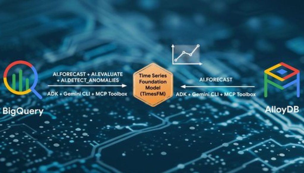
We are thrilled to announce the integration of TimesFM into our leading data platforms, BigQuery and AlloyDB. This brings the power of large-scale, pre-trained forecasting models directly to your data within the Google Data Cloud, enabling you to predict future trends with unprecedented ease and accuracy.
TimesFM is a powerful time-series foundation model developed by Google Research, pre-trained on a vast dataset of over 400 billion real-world time-points. This extensive training allows TimesFM to perform “zero-shot” forecasting, meaning it can generate accurate predictions for your specific data without needing to be retrained. This dramatically simplifies the process of creating and deploying forecasting models, saving you time and resources.
Now, let’s dive into what this means for you in BigQuery and AlloyDB.
TimesFM in BigQuery
We launched the AI.FORECAST function in preview at Google Cloud Next ‘25. Today, we are announcing:
- AI.FORECAST and AI.EVALUATE are now Generally Available (GA).
- AI.DETECT_ANOMALIES is now in Public Preview.
- AI.FORECAST is supported in multiple open-source frameworks, including
Let’s take a look at these in greater depth.
AI.FORECAST and AI.EVALUATE
The GA launch includes major upgrades:
-
TimesFM 2.5 is now supported. By specifying `model => “TimesFM 2.5”`, you can use the latest TimesFM model to achieve better forecasting accuracy and lower latency.
-
AI.FORECAST supports dynamic context windows up to 15K: Multiple context windows from 64 to 15K are supported, by specifying `context_window`. If not specified, a context window is selected to match the time series input size.
-
AI.FORECAST supports displaying historical data: Displaying historical data together with forecasts is supported by setting `output_historical_time_series` to true. The option enhances usability by enabling easier and better visualizations.
-
We add AI.EVALUATE for model evaluation. Users can specify the actual data to evaluate the accuracy of the forecasted value.
In this example, you can use the TimesFM 2.5 model and specify the context window = 1024 in AI.FORECAST to use the latest 1024 points as the history data. You can specify output_historical_time_series = true to display historical data together with the forecasts.
- code_block
- <ListValue: [StructValue([(‘code’, “WITH citibike_trips AS (rn SELECT EXTRACT(DATE FROM starttime) AS date, COUNT(*) AS num_tripsrn FROM `bigquery-public-data.new_york.citibike_trips` GROUP BY date)rnSELECT *rnFROMrn AI.FORECAST(rn TABLE citibike_trips, — History Tablern data_col => ‘num_trips’,rn timestamp_col => ‘date’,rn horizon => 300,rn output_historical_time_series => TRUE,rn model => ‘TimesFM 2.5’,rn context_window => 1024);”), (‘language’, ”), (‘caption’, <wagtail.rich_text.RichText object at 0x7f7c0c24f5e0>)])]>
The first 10 days forecasted values are:

You can also visualize the results by clicking the `Visualization` tab. The results should be similar to:

In this example of AI.EVALUATE, you can use the data before “2016-08-01” as history to evaluate the forecasted bike trips against the actual data after “2016-08-01”:
- code_block
- <ListValue: [StructValue([(‘code’, ‘WITH citibike_trips AS (rn SELECT EXTRACT(DATE FROM starttime) AS date, usertype, COUNT(*) AS num_tripsrn FROM `bigquery-public-data.new_york.citibike_trips` GROUP BY date, usertype)rnSELECT * rnFROMrn AI.EVALUATE(rn (SELECT * FROM citibike_trips WHERE date < ‘2016-08-01’), — History time seriesrn (SELECT * FROM citibike_trips WHERE date >= ‘2016-08-01’), — Actual time seriesrn data_col => ‘num_trips’,rn timestamp_col => ‘date’,rn id_cols => [“usertype”]);’), (‘language’, ”), (‘caption’, <wagtail.rich_text.RichText object at 0x7f7c0c24ff10>)])]>
The SQL generates evaluation metrics based on each `usertype`:

AI.DETECT_ANOMALIES
The addition of AI.DETECT_ANOMALIES lets you specify the target data to detect anomalies against the forecasted value.
In this example of AI.DETECT_ANOMALIES, you can use the data before “2016-08-01” as history to detect anomalies in the target data after “2016-08-01”:
- code_block
- <ListValue: [StructValue([(‘code’, ‘WITH citibike_trips AS (rn SELECT EXTRACT(DATE FROM starttime) AS date, usertype, COUNT(*) AS num_tripsrn FROM `bigquery-public-data.new_york.citibike_trips` GROUP BY date, usertype)rnSELECT * rnFROMrn AI.DETECT_ANOMALIES(rn (SELECT * FROM citibike_trips WHERE date < ‘2016-08-01’), — History time series rn (SELECT * FROM citibike_trips WHERE date >= ‘2016-08-01’), — Target time seriesrn data_col => ‘num_trips’,rn timestamp_col => ‘date’,rn id_cols => [“usertype”]);’), (‘language’, ”), (‘caption’, <wagtail.rich_text.RichText object at 0x7f7c0c24f280>)])]>
The SQL generates the anomalies per usertype for each data point that is after “2016-08-01”, an example of 10 rows of results are:

TimesFM in AlloyDB
AI.FORECAST is now available in AlloyDB in preview. AlloyDB provides built-in support for TimesFM for predictions directly from inside of AlloyDB. This enables you to make predictions leveraging operational and analytical data for use cases such as sales forecasting, inventory demand prediction, or operational load modeling, without needing to export data.

Forecasting sales with AlloyDB
Let’s walk through an example of how you can forecast sales leveraging data stored in AlloyDB. Traditionally you would have to set up and maintain an ETL pipeline to extract data from AlloyDB, pull it into a data science environment, potentially deploy a forecasting model, run predictions for the model and store them. But for time-sensitive applications, these steps can be costly.
Instead, suppose you are leveraging AlloyDB for your operational workloads. You have stored sales, stock and price data, along with metadata, in a table retail_sales. You know what happened last week in terms of sales, but you want to predict what will happen next week so that you can plan accordingly to the demand.
With AlloyDB’s latest integration, you can get started with just two simple steps.
1. Register the model. Register the TimesFM model as a model endpoint within AlloyDB’s model endpoint management in order to point to the Vertex AI endpoint where the model is hosted. This allows AlloyDB to securely send time-series data to the model and receive predictions back. Here we point to a TimesFM model deployed on Vertex AI and choose a model id “timesfm_v2”.
- code_block
- <ListValue: [StructValue([(‘code’, “CALLrn ai.create_model(rn model_id => ‘timesfm_v2’,rn model_type => ‘ts_forecasting’,rn model_provider => ‘google’,rn model_qualified_name => ‘timesfm_v2’,rn model_request_url => ‘https://<REGION>-aiplatform.googleapis.com/v1/projects/<PROJECT_ID>/locations/<REGION>/endpoints/<ENDPOINT_ID>:predict’ — endpoint in Vertex AI Model Gardenrn);”), (‘language’, ”), (‘caption’, <wagtail.rich_text.RichText object at 0x7f7c0c24f490>)])]>
2. Generate Predictions with AI.FORECAST.Once the model is registered, you can start leveraging the AI.FORECAST function. This function takes your time-series data and prediction parameters (like the forecast horizon) and returns the forecasted values.
In this example, we’ll forecast the next 11 days of sales based on the sales data stored in our database with a confidence level of .80.
- code_block
- <ListValue: [StructValue([(‘code’, “SELECT * FROM ai.forecast(rn model_id => ‘timesfm_v2’,rn source_table => ‘retail_sales’,rn data_col => ‘sales’,rn timestamp_col => ‘timestamp’,rn horizon => 11,rn conf_level => 0.8rn);”), (‘language’, ”), (‘caption’, <wagtail.rich_text.RichText object at 0x7f7c0c24f430>)])]>

This integrated approach means you can keep your data securely within your high-performance AlloyDB instance and immediately leverage Google’s state-of-the-art forecasting capabilities. The low latency of AlloyDB, combined with the zero-shot power of TimesFM, makes real-time predictive analytics a reality for your operational workloads. Read more about our integration in this blog post.
AI.FORECAST in Agents and MCP
In addition to supporting TimesFM (AI.FORECAST) via a SQL interface, you can leverage TimesFM’s prediction capabilities on BigQuery and AlloyDB via agentic interfaces such as Agent Development Kit (ADK), MCP toolbox for Databases, and the Gemini CLI extension for Google Data Cloud.
Use BigQuery built-in forecast tool
This blog post shows you how to write your agent with ADK’s built-in BigQuery forecast tool (via TimesFM) to do the forecast task with your data. Here is a quick peek of how you can run forecasting task via natural language with an agent built with ADK:

This blog post can walk you through how to install and configure the MCP extension and use the BigQuery forecast tool in the Gemini CLI.
Take the next step
The TimesFM model is now generally available in BigQuery. For more details, please see the tutorial and the documentation for AI.FORECAST, AI.EVALUTE and AI.DETECT_ANOMALIES. You can also get started on TimesFM today on AlloyDB.
Read More for the details.


