GCP – Building a Production Multimodal Fine-Tuning Pipeline

Looking to fine-tune multimodal AI models for your specific domain but facing infrastructure and implementation challenges? This guide demonstrates how to overcome the multimodal implementation gap using Google Cloud and Axolotl, with a complete hands-on example fine-tuning Gemma 3 on the SIIM-ISIC Melanoma dataset. Learn how to scale from concept to production while addressing the typical challenges of managing GPU resources, data preparation, and distributed training.

Filling in the Gap

Organizations across industries are rapidly adopting multimodal AI to transform their operations and customer experiences. Gartner analysts predict 40% of generative AI solutions will be multimodal (text, image, audio and video) by 2027, up from just 1% in 2023, highlighting the accelerating demand for solutions that can process and understand multiple types of data simultaneously.

Healthcare providers are already using these systems to analyze medical images alongside patient records, speeding up diagnosis. Retailers are building shopping experiences where customers can search with images and get personalized recommendations. Manufacturing teams are spotting quality issues by combining visual inspections with technical data. Customer service teams are deploying agents that process screenshots and photos alongside questions, reducing resolution times.

Multimodal AI applications powerfully mirror human thinking. We don’t experience the world in isolated data types – we combine visual cues, text, sound, and context to understand what’s happening. Training multimodal models on your specific business data helps bridge the gap between how your teams work and how your AI systems operate.

Key challenges organizations face in production deployment

Moving from prototype to production with multimodal AI isn’t easy. PwC survey data shows that while companies are actively experimenting, most expect fewer than 30% of their current experiments to reach full scale in the next six months. The adoption rate for customized models remains particularly low, with only 20-25% of organizations actively using custom models in production.

The following technical challenges consistently stand in the way of success:

Infrastructure complexity: Multimodal fine-tuning demands substantial GPU resources – often 4-8x more than text-only models. Many organizations lack access to the necessary hardware and struggle to configure distributed training environments efficiently.

Data preparing hurdles: Preparing multimodal training data is fundamentally different from text-only preparation. Organizations struggle with properly formatting image-text pairs, handling diverse file formats, and creating effective training examples that maintain the relationship between visual and textual elements.

Training workflow management: Configuring and monitoring distributed training across multiple GPUs requires specialized expertise most teams don’t have. Parameter tuning, checkpoint management, and optimization for multimodal models introduce additional layers of complexity.

These technical barriers create what we call “the multimodal implementation gap” – the difference between recognizing the potential business value and successfully delivering it in production.

How Google Cloud and Axolotl together solve these challenges

Our collaboration brings together complementary strengths to directly address these challenges. Google Cloud provides the enterprise-grade infrastructure foundation necessary for demanding multimodal workloads. Our specialized hardware accelerators such as NVIDIA B200 Tensor Core GPUs and Ironwood are optimized for these tasks, while our managed services like Google Cloud Batch, Vertex AI Training, and GKE Autopilot minimize the complexities of provisioning and orchestrating multi-GPU environments. This infrastructure seamlessly integrates with the broader ML ecosystem, creating smooth end-to-end workflows while maintaining the security and compliance controls required for production deployments.

Axolotl complements this foundation with a streamlined fine-tuning framework that simplifies implementation. Its configuration-driven approach abstracts away technical complexity, allowing teams to focus on outcomes rather than infrastructure details. Axolotl supports multiple open source and open weight foundation models and efficient fine-tuning methods like QLoRA. This framework includes optimized implementations of performance-enhancing techniques, backed by community-tested best practices that continuously evolve through real-world usage.

Together, we enable organizations to implement production-grade multimodal fine-tuning without reinventing complex infrastructure or developing custom training code. This combination accelerates time-to-value, turning what previously required months of specialized development into weeks of standardized implementation.

Solution Overview

Our multimodal fine-tuning pipeline consists of five essential components:

1. Foundational model: Choose a base model that meets your task requirements. Axolotl supports a variety of open source and open weight multimodal models including Llama 4, Pixtral, LLaVA-1.5, Mistral-Small-3.1, Qwen2-VL, and others. For this example, we’ll use Gemma 3, our latest open and multimodal model family.
2. Data preparation: Create properly formatted multimodal training data that maintains the relationship between images and text. This includes organizing image-text pairs, handling file formats, and splitting data into training/validation sets.
3. Training configuration: Define your fine-tuning parameters using Axolotl’s YAML-based approach, which simplifies settings for adapters like QLoRA, learning rates, and model-specific optimizations.
4. Infrastructure orchestration: Select the appropriate compute environment based on your scale and operational requirements. Options include Google Cloud Batch for simplicity, Google Kubernetes Engine for flexibility, or Vertex AI Custom Training for MLOps integration.
5. Production integration: Streamlined pathways from fine-tuning to deployment.

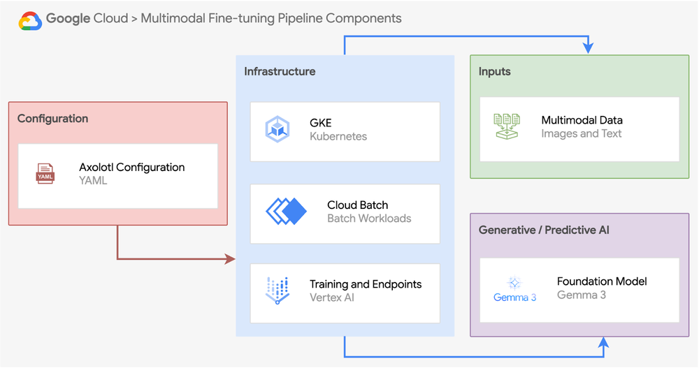
The pipeline structure above represents the conceptual components of a complete multimodal fine-tuning system. In our hands-on example later in this guide, we’ll demonstrate these concepts through a specific implementation tailored to the SIIM-ISIC Melanoma dataset, using GKE for orchestration. While the exact implementation details may vary based on your specific dataset characteristics and requirements, the core components remain consistent.

Selecting the Right Google Cloud Environment

Google Cloud offers multiple approaches to orchestrating multimodal fine-tuning workloads. Let’s explore three options with different tradeoffs in simplicity, flexibility, and integration:

Google Cloud Batch

Google Cloud Batch is best for teams seeking maximum simplicity for GPU-intensive training jobs with minimal infrastructure management. It handles all resource provisioning, scheduling, and dependencies automatically, eliminating the need for container orchestration or complex setup. This fully managed service balances performance and cost effectiveness, making it ideal for teams who need powerful computing capabilities without operational overhead.

Vertex AI Custom Training

Vertex AI Custom Training is best for teams prioritizing integration with Google Cloud’s MLOps ecosystem and managed experiment tracking. Vertex AI Custom Training jobs automatically integrate with Experiments for tracking metrics, the Model Registry for versioning, Pipelines for workflow orchestration, and Endpoints for deployment.

Google Kubernetes Engine (GKE)

GKE is best for teams seeking flexible integration with containerized workloads. It enables unified management of training jobs alongside other services in your container ecosystem while leveraging Kubernetes’ sophisticated scheduling capabilities. GKE offers fine-grained control over resource allocation, making it ideal for complex ML pipelines. For our hands-on example, we’ll use GKE in Autopilot mode, which maintains these integration benefits while Google Cloud automates infrastructure management including node provisioning and scaling. This lets you focus on your ML tasks rather than cluster administration, combining the flexibility of Kubernetes with the operational simplicity of a managed service.

Take a look at our code sample here for a complete implementation that demonstrates how to orchestrate a multimodal fine-tuning job on GKE:

This repository includes ready-to-use Kubernetes manifests for deploying Axolotl training jobs on GKE in Autopilot mode, covering automated cluster setup with GPUs, persistent storage configuration, job specifications, and monitoring integration.

Hands-on example: Fine-tuning Gemma 3 on the SIIM-ISIC Melanoma dataset

This section involves dermoscopic images of skin lesions with labels indicating whether they are malignant or benign. With melanoma accounting for 75% of skin cancer deaths despite its relative rarity, early and accurate detection is critical for patient survival. By applying multimodal AI to this challenge, we unlock the potential to help dermatologists improve diagnostic accuracy and potentially save lives through faster, more reliable identification of dangerous lesions. So, let’s walk through a complete example fine-tuning Gemma 3 on the SIIM-ISIC Melanoma Classification dataset.

For this implementation, we’ll leverage GKE in Autopilot mode to orchestrate our training job and monitoring, allowing us to focus on the ML workflow while Google Cloud handles the infrastructure management.

Data Preparation

The SIIM-ISIC Melanoma Classification dataset requires specific formatting for multimodal fine-tuning with Axolotl. Our data preparation process involves two main steps: (1) efficiently transferring the dataset to Cloud Storage using Storage Transfer Service, and (2) processing the raw data into the format required by Axolotl. To start, transfer the dataset.

Create a TSV file that contains the URLs for the ISIC dataset files:

Create a bucket for your dataset:

Upload the TSV file to your Cloud Storage bucket:

Set up appropriate IAM permissions for the Storage Transfer Service:

Set up a storage transfer job using the URL list:

1. Navigate to Cloud Storage > Transfer
2. Click “Create Transfer Job”
3. Select “URL list” as Source type and “Google Cloud Storage” as Destination type
4. Enter the path to your TSV file: gs://<GCS_BUCKET_NAME>/melanoma_dataset_urls.tsv
5. Select your destination bucket
6. Use the default job settings and click Create

The transfer will download approximately 32GB of data from the ISIC Challenge repository directly to your Cloud Storage bucket. Once the transfer is complete, you’ll need to extract the ZIP files before proceeding to the next step where we’ll format this data for Axolotl. See the notebook in the Github repository here for a full walk-through demonstration on how to format the data for Axolotl.

Preparing Multimodal Training Data

For multimodal models like Gemma 3, we need to structure our data following the extended chat_template format, which defines conversations as a series of messages with both text and image content.

Below is an example of a single training input example:

We split the data into training (80%), validation (10%), and test (10%) sets, while maintaining the class distribution in each split using stratified sampling.

This format allows Axolotl to properly process both the images and their corresponding labels, maintaining the relationship between visual and textual elements during training.

Creating the Axolotl Configuration File

Next, we’ll create a configuration file for Axolotl that defines how we’ll fine-tune Gemma 3. We’ll use QLoRA (Quantized Low-Rank Adaptation) with 4-bit quantization to efficiently fine-tune the model while keeping memory requirements manageable. While A100 40GB GPUs have substantial memory, the 4-bit quantization with QLoRA allows us to train with larger batch sizes or sequence lengths if needed, providing additional flexibility for our melanoma classification task. The slight reduction in precision is typically an acceptable tradeoff, especially for fine-tuning tasks where we’re adapting a pre-trained model rather than training from scratch.

This configuration sets up QLoRA fine-tuning with parameters optimized for our melanoma classification task. Next, we’ll set up our GKE Autopilot environment to run the training.

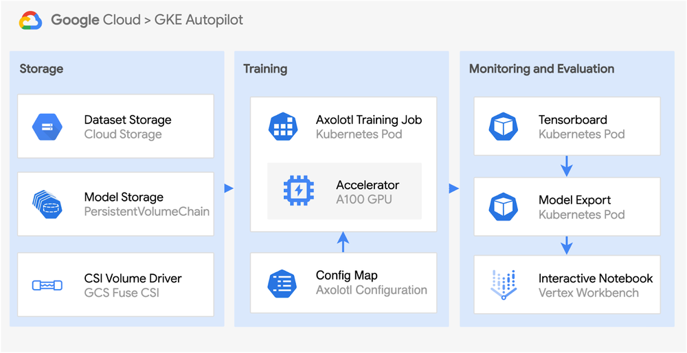
Setting up GKE Autopilot for GPU Training

Now that we have our configuration file ready, let’s set up the GKE Autopilot cluster we’ll use for training. As mentioned earlier, Autopilot mode lets us focus on our ML task while Google Cloud handles the infrastructure management.

Let’s create our GKE Autopilot cluster:

Now set up Workload Identity Federation for GKE to securely authenticate with Google Cloud APIs without using service account keys:

Now create a PersistentVolumeClaim for our model outputs. In Autopilot mode, Google Cloud manages the underlying storage classes, so we don’t need to create our own:

Apply the PVC configuration:

Deploying the Training Job to GKE Autopilot

In Autopilot mode, we specify our GPU requirements using annotations and resource requests within the Pod template section of our Job definition. We’ll create a Kubernetes Job that requests a single A100 40GB GPU:

Create a ConfigMap with our Axolotl configuration:

Create a Secret with Hugging Face credentials:

Apply training job YAML to start the training process:

Monitor the Training Process

Fetch the pod name to monitor progress:

Set up TensorBoard to visualize training metrics:

Deploy TensorBoard:

Model Export and Evaluation Setup

After training completes, we need to export our fine-tuned model and evaluate its performance against the base model. First, let’s export the model from our training environment to Cloud Storage:

Create a pod to export the model:

After creating the model-export.yaml file, apply it:

This will start the export process, which copies the fine-tuned model from the Kubernetes PersistentVolumeClaim to your Cloud Storage bucket for easier access and evaluation.

Once exported, we have several options for evaluating our fine-tuned model. You can deploy both the base and fine-tuned models to their own respective Vertex AI Endpoints for systematic testing via API calls, which works well for high-volume automated testing and production-like evaluation. Alternatively, for exploratory analysis and visualization, a GPU-enabled notebook environment such as a Vertex Workbench Instance or Colab Enterprise offers significant advantages, allowing for real-time visualization of results, interactive debugging, and rapid iteration on evaluation metrics.

In this example, we use a notebook environment to leverage its visualization capabilities and interactive nature. Our evaluation approach involves:

• Loading both the base and fine-tuned models

• Running inference on a test set of dermatological images from the SIIM-ISIC dataset

• Computing standard classification metrics (accuracy, precision, recall, etc.)

• Analyzing the confusion matrices to understand error patterns

• Generating visualizations to highlight performance differences

For the complete evaluation code and implementation details, check out our evaluation notebook in the GitHub repository. 

Performance Results

Our evaluation demonstrated that domain-specific fine-tuning can transform a general-purpose multimodal model into a much more effective tool for specialized tasks like medical image classification. The improvements were significant across multiple dimensions of model performance.

The most notable finding was the base model’s tendency to over-diagnose melanoma. It showed perfect recall (1.000) but extremely poor specificity (0.011), essentially labeling almost every lesion as melanoma. This behavior is problematic in clinical settings where false positives lead to unnecessary procedures, patient anxiety, and increased healthcare costs.

Fine-tuning significantly improved the model’s ability to correctly identify benign lesions, reducing false positives from 3,219 to 1,438. While this came with a decrease in recall (from 1.000 to 0.603), the tradeoff resulted in much better overall diagnostic capability, with balanced accuracy improving substantially.

In our evaluation, we also included results from the newly announced MedGemma—a collection of Gemma 3 variants trained specifically for medical text and image comprehension recently released at Google I/O. These results further contribute to our understanding of how different model starting points affect performance on specialized healthcare tasks.

Below we can see the performance metrics across all three models:

Accuracy jumped from a mere 0.028 for base Gemma 3 to 0.559 for our tuned Gemma 3 model, representing an astounding 1870.2% improvement. MedGemma achieved 0.893 accuracy without any task-specific fine-tuning—a 3048.9% improvement over the base model and substantially better than our custom-tuned version.

While precision saw a significant 34.2% increase in our tuned model (from 0.018 to 0.024), MedGemma delivered a substantial 112.5% improvement (to 0.038). The most remarkable transformation occurred in specificity—the model’s ability to correctly identify non-melanoma cases. Our tuned model’s specificity increased from 0.011 to 0.558 (a 4947.2% improvement), while MedGemma reached 0.906 (an 8088.9% improvement over the base model).

These numbers highlight how fine-tuning helped our model develop a more nuanced understanding of skin lesion characteristics rather than simply defaulting to melanoma as a prediction. MedGemma’s results demonstrate that starting with a medically-trained foundation model provides considerable advantages for healthcare applications.

The confusion matrices further illustrate these differences:

Looking at the base Gemma 3 matrix (left), we can see it correctly identified all 58 actual positive cases (perfect recall) but also incorrectly classified 3,219 negative cases as positive (poor specificity). Our fine-tuned model (center) shows a more balanced distribution, correctly identifying 1,817 true negatives while still catching 35 of the 58 true positives. MedGemma (right) shows strong performance in correctly identifying 2,948 true negatives, though with more false negatives (46 missed melanoma cases) than the other models.

To illustrate the practical impact of these differences, let’s examine a real example, image ISIC_4908873, from our test set:

The base model incorrectly classified it as melanoma. Its rationale focused on general warning signs, citing its “significant variation in color,” “irregular, poorly defined border,” and “asymmetry” as definitive indicators of malignancy, without fully contextualizing these within broader benign patterns.

In contrast, our fine-tuned model correctly identified it as benign. While acknowledging a “heterogeneous mix of colors” and “irregular borders,” it astutely noted that such color mixes can be “common in benign nevi.” Crucially, it interpreted the lesion’s overall “mottled appearance with many small, distinct color variations” as being “more characteristic of a common mole rather than melanoma.”

Interestingly, MedGemma also misclassified this lesion as melanoma, stating, “The lesion shows a concerning appearance with irregular borders, uneven coloration, and a somewhat raised surface. These features are suggestive of melanoma. Yes, this appears to be malignant melanoma.” Despite MedGemma’s overall strong statistical performance, this example illustrates that even domain-specialized models can benefit from task-specific fine-tuning for particular diagnostic challenges.

These results underscore a critical insight for organizations building domain-specific AI systems: while foundation models provide powerful starting capabilities, targeted fine-tuning is often essential to achieve the precision and reliability required for specialized applications. The significant performance improvements we achieved—transforming a model that essentially labeled everything as melanoma into one that makes clinically useful distinctions—highlight the value of combining the right infrastructure, training methodology, and domain-specific data.

MedGemma’s strong statistical performance demonstrates that starting with a domain-focused foundation model significantly improves baseline capabilities and can reduce the data and computation needed for building effective medical AI applications. However, our example case also shows that even these specialized models would benefit from task-specific fine-tuning for optimal diagnostic accuracy in clinical contexts.

Next steps for your multimodal journey

By combining Google Cloud’s enterprise infrastructure with Axolotl’s configuration-driven approach, you can transform what previously required months of specialized development into weeks of standardized implementation, bringing custom multimodal AI capabilities from concept to production with greater efficiency and reliability.

For deeper exploration, check out these resources:

• Axolotl Multimodal Guide

• GKE Documentation

• Google Cloud Batch Documentation

• Vertex Custom Training Documentation

• Gemma 3 Technical Documentation

• Health AI Developer Foundations

• MedGemma on Hugging Face